The Analysis view
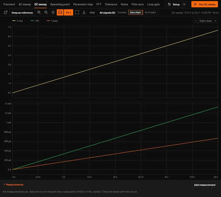
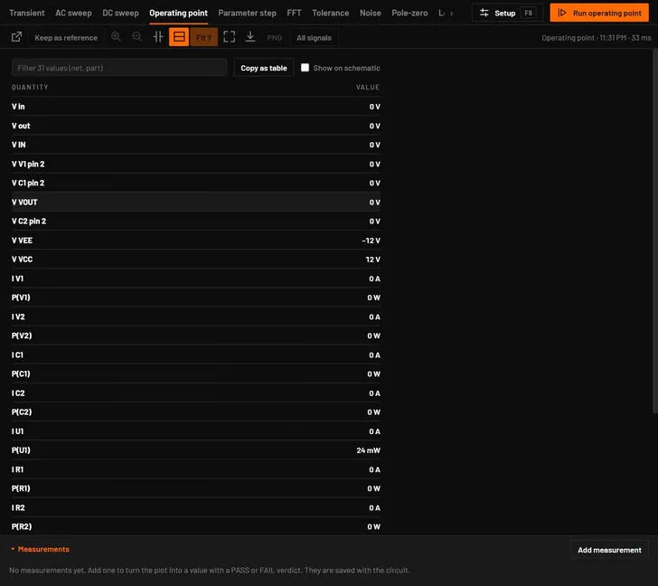
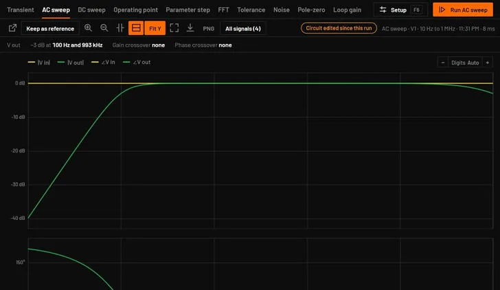
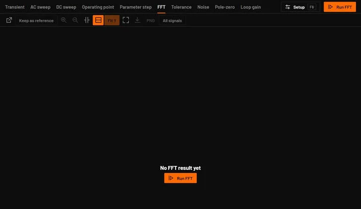
The Analysis view shows the result of the analysis tab you have open, with a caption that names the run. When the window is too narrow for every tab, the strip scrolls and shows ‹ and › arrows, and the open tab is kept in view. Each tab keeps its own last result, per circuit, also across circuit tabs: an AC result is still there after you ran a DC sweep, and a result that arrives after you switched tabs goes to the tab that ran it. A tab that hasn't been run says No operating point result yet (or the name of its analysis) with a Run button. When you change parts or wires after a run, a Circuit edited since this run chip appears. Run again for the current circuit. The Bode dock tab shows the AC result. While a run is going, the plot area says Simulating with a Cancel button. Ctrl+2 shows it alone, Ctrl+3 under the schematic.
 1234567
29.1The bars
| Bar | Contents |
|---|---|
| 1 2 Top | The analysis tabs, a line such as Transient · 4 002 points · 37 ms, Setup F6 and Run, which becomes Cancel during a run. |
| Progress | While running: a bar and "Step 5 of 6: Simulating in ngspice · 42 % · 6 s · about 30 s left". A vendor run that heads for a big result shows its memory warning here, with Stop and keep less and Keep going. |
| Error | After a failure: Simulation failed: with the reason, and Dismiss. |
| 3 Tools | Pop out, Cursors, One pane per unit, Fit, Export CSV, PNG, All signals, Remove probed traces. |
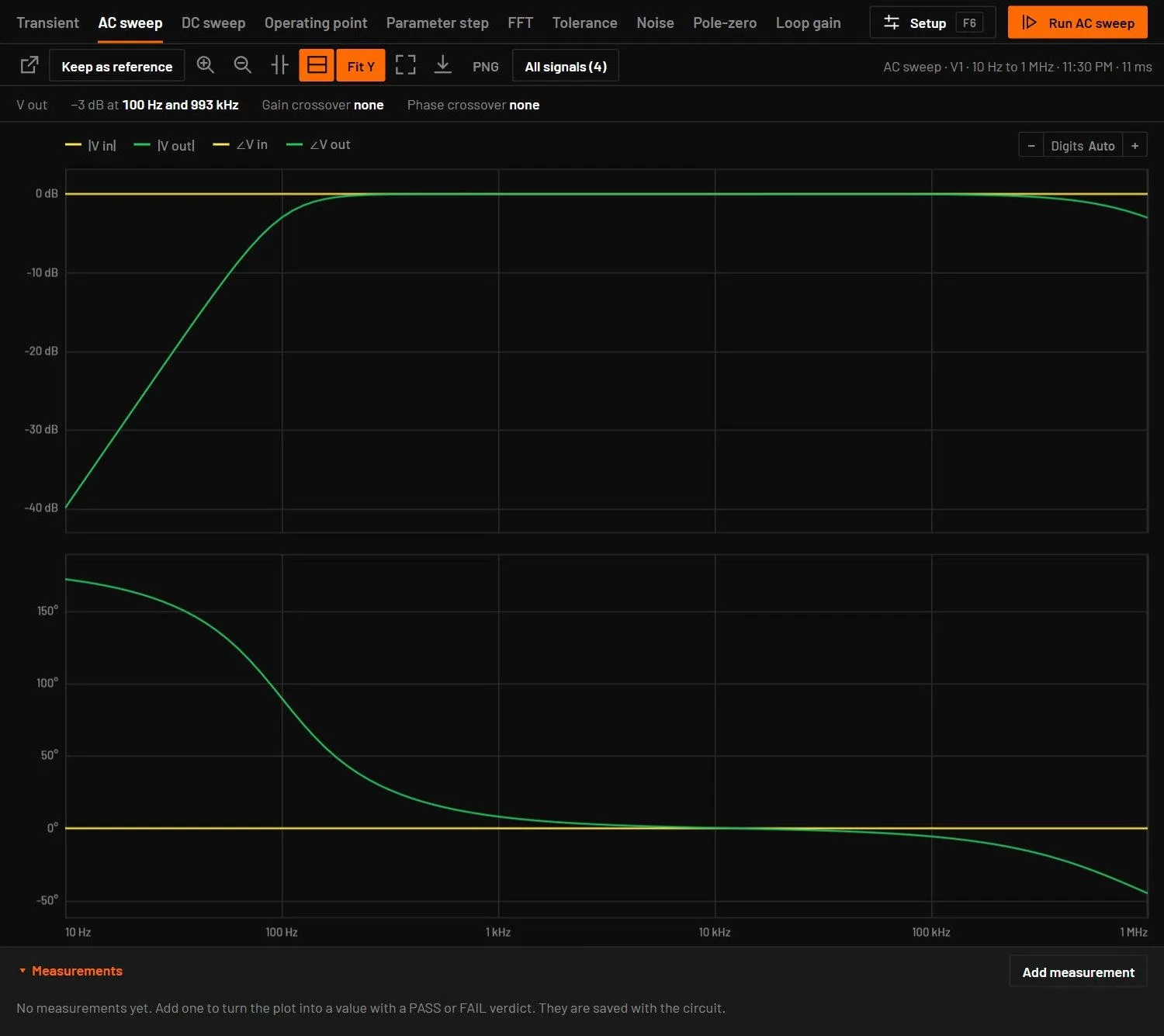
| 4 Margins | AC results only: −3 dB points, crossovers, phase and gain margin. |
| 5 Legend | One entry per trace. Hold the pointer over a name to light up its net or part on the schematic. The − Digits Auto + control at its right end sets the readout digits (Axis labels and readout digits). In a narrow window the toolbar row wraps instead of running under the Inspector. |
29.2The tools
| Tool | What it does |
|---|---|
| Pop out / Dock back | Moves the Analysis view into its own window. The main window then says where it is and offers to bring it back. |
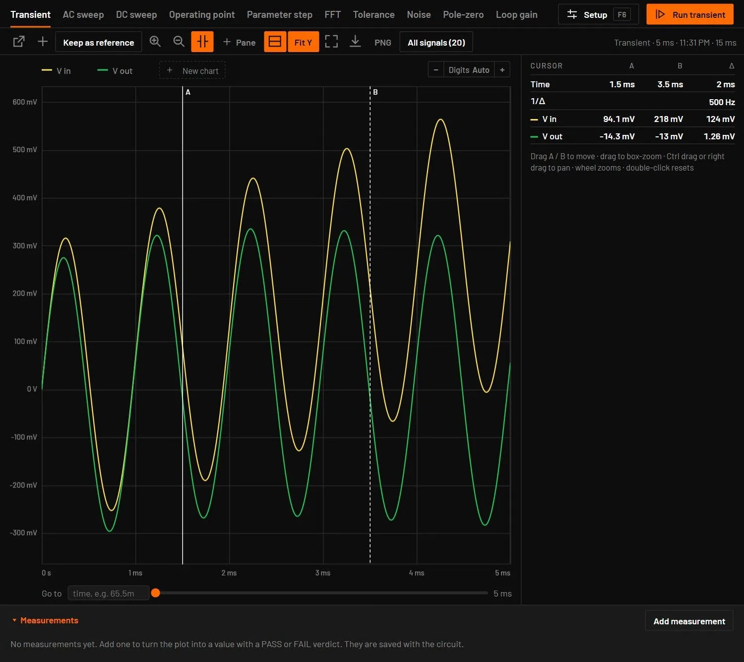
| Cursors | Cursor lines A and B with a readout (Cursors). |
| One pane per unit | On by default: volts, amps and decibels on separate panes with a shared time axis. Off: all traces on one pane. |
| Fit | Resets the zoom. |
| Fit Y | On by default. Each pane's vertical axis fits the part of the run you have zoomed to, and follows zoom and pan. The scope's flags Max, Fixed and Manual show, and Fit Y off when it is off. Turn it off to keep the range of the whole run. It also sits in the plot menu under Scale, as Fit Y to the zoomed view, and is remembered. |
| Export CSV | Saves the data: transient.csv, bode.csv or operating-point.csv. Up to 200 000 rows it saves at once. In the desktop app a longer run writes every row, in pieces of about 4 MB, so a result of millions of rows saves without filling memory. The desktop asks where to save. |
| PNG | Saves the plot with its legend as a picture. |
| All signals / Probes only | Works on any run. Every signal is kept at every step; only Keep less, or the browser version (its engine holds at most 240 MB), keeps the signals that are no probe as the lowest and highest value of short time slices (a spike shorter than a slice still shows). Switching between All signals and Probes only never runs the analysis again. All signals opens a signal list beside the plot: a filter (several words, all must match), V or I, a click on a row to plot it or take it off, and Shift or Ctrl click to pick several. Each row shows the value at the pointer, else at the playhead, else at the end of the run. Drag rows onto a chart, or onto New chart. Delete takes a trace off. With more than 16 traces the hover box lists the ten nearest the pointer, and a plot of 100 or more traces stays quick. |
| Remove N probed traces | Removes the traces you added by clicking the schematic. |
29.3Measurements
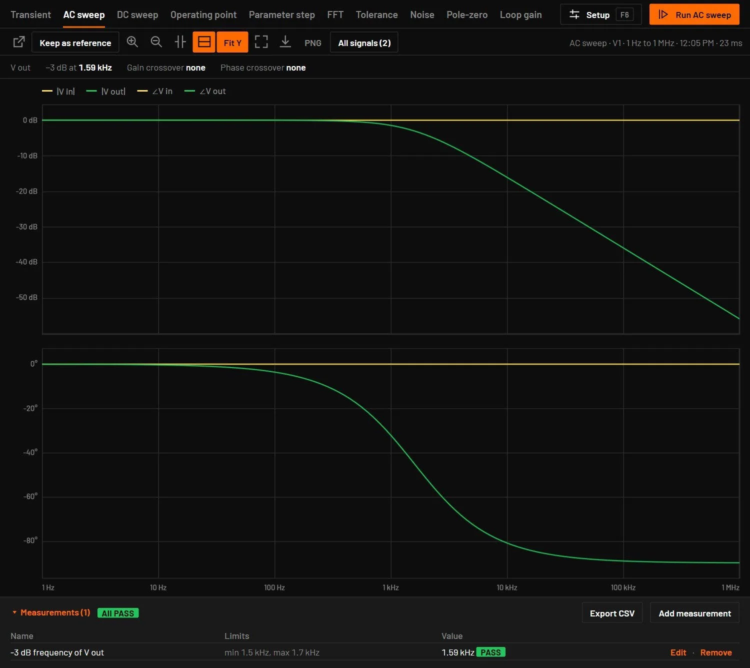
Under the plot of a transient, DC sweep, AC sweep, operating point or parameter step, the Measurements panel lists named measurements with a value and, when limits are set, PASS or FAIL. Add measurement opens the editor. Measurements are saved in the circuit, evaluated after every run, shown for every value of a parameter step, and judged in every run of a tolerance analysis. Export CSV saves the table.
| Measurement | What it reads |
|---|---|
| Minimum, maximum, average, RMS, peak to peak, final value | The window From to To, or the whole run when empty. Average and RMS are time-weighted. |
| Value at | One time (or swept value), interpolated. |
| Frequency, duty cycle | Rising edges through the middle level, with 10 % hysteresis. |
| Rise time, fall time | Between the lower and upper threshold (default 10 % and 90 % of the step) on the first edge. |
| Overshoot | Percent past the final value after a step. |
| Settling time | From the window start until the output stays within a band (default 2 % of the step) of its final value. |
| Ripple | Peak to peak after a start time. Set From past the start-up. |
| Delay between signals | From the first signal crossing its middle level to the second one doing so. |
| Efficiency | Average output power over average input power, in percent. Both are expressions of probe labels, for example "Vout"*"Iout" over -"Vin"*"Iin". |
| Gain at, phase at | An AC result at one frequency. |
| -3 dB frequency, unity-gain frequency | An AC result. |
| Phase margin, gain margin | An AC result that is a loop gain. A loop whose low-frequency phase starts near 180 degrees is handled. |
Rise, fall, overshoot and settling take the first and last value of the window as the two levels when the window holds one clean step (they differ by at least half the swing). Otherwise rise and fall use the minimum and maximum, and overshoot and settling say the window holds no single step. Start the window before the edge and end it after the output has settled. A limit on a value that cannot be measured counts as a FAIL and the row says why. Total harmonic distortion is not a measurement here. It is in the FFT.
29.4Keep as reference
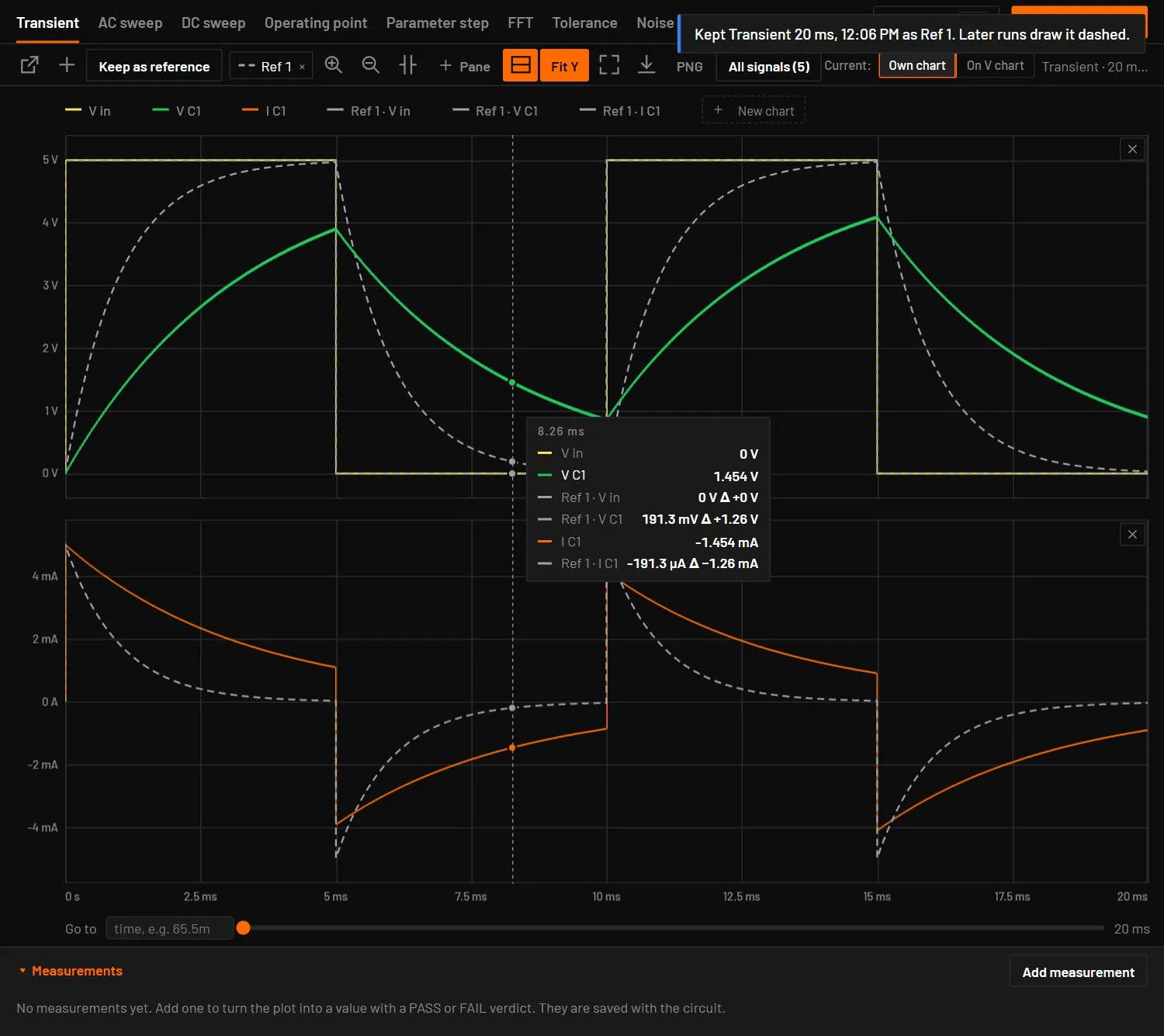
Keep as reference in the Analysis toolbar keeps the transient, DC sweep or AC sweep on screen. Later runs of the same kind draw it dashed behind their own traces, and the hover readout shows the difference of each trace to it. Up to five runs are kept at once, as Ref 1 to Ref 5, each in its own colour: its traces are named Ref 2 · V out. Each kept run has a chip next to the button: click it to hide or show that run, and its × deletes it. A sixth kept run takes the place of the oldest. Opening or starting another circuit clears them. They are not saved with the circuit, and the report draws the last one shown.
29.5Fit Y in the Analysis view
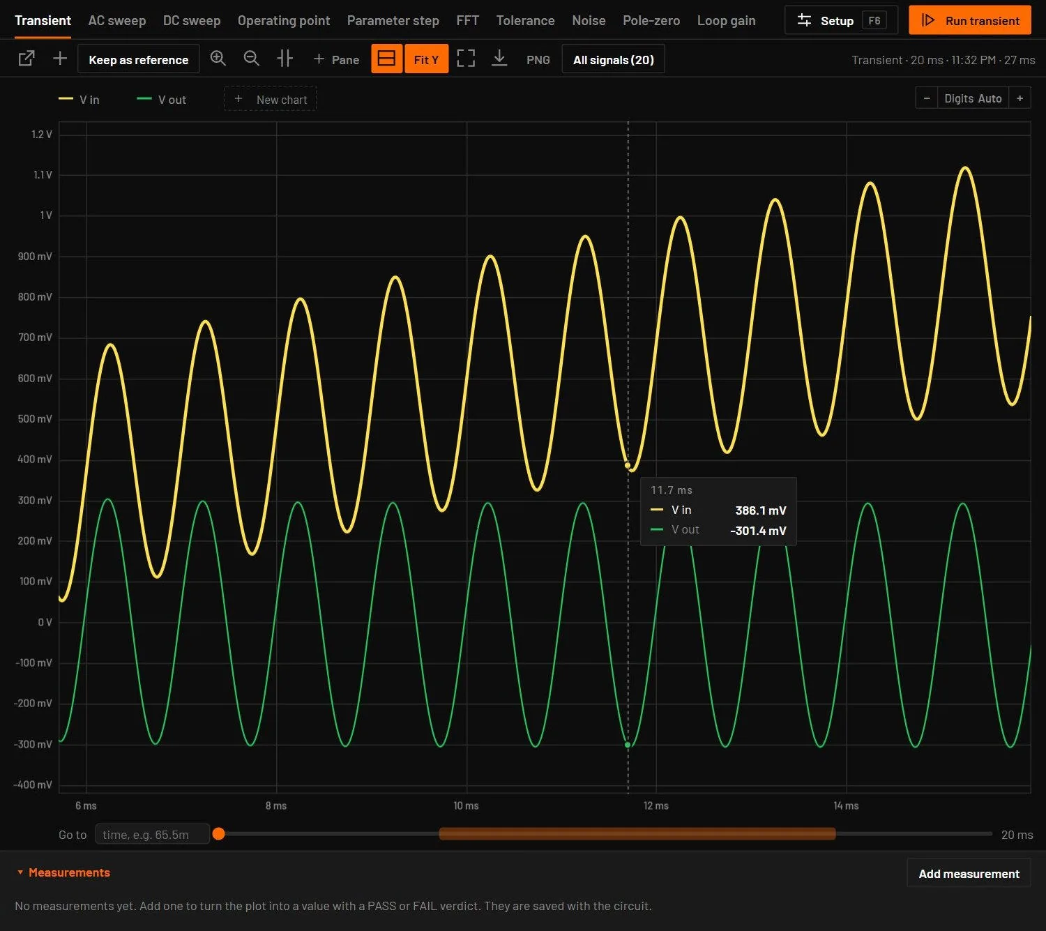
With Fit Y on, zooming in time also rescales each pane vertically, so a small part of a large signal fills the pane. The button in the plot toolbar is lit, and a flag in the corner of the plot names the scale in use.
29.6Notes about a result
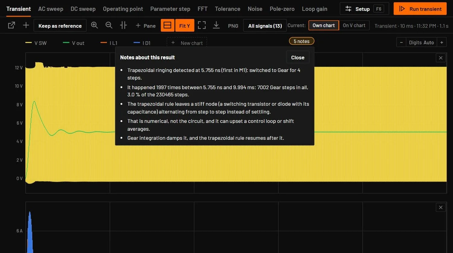
Warnings about a result, such as a node held only by leakage or a switch to Gear after ringing, are one small chip at the end of the plot's legend, for example 4 notes. Click it to read them in a panel. Close, Esc or a click outside closes it. A note never covers the traces.
29.7Newton predictor
(also in Simulation setup, Transient tab, off by default) starts each time step's Newton solve from a point extrapolated from the last two steps. Measured on 92 circuits it is not faster on most of them (up to 1.55x on smooth analog circuits, 1.14x on a 578-part board) and changes results slightly: typically under 0.001 %, up to 6 % of a signal's swing near switching edges. Leave it off unless a long analog run needs it. A run made with it says so with a Newton predictor on chip beside its trace names, the measured differences in the chip’s tooltip and in the notes. bspice tran --predictor does the same, and verify always runs exact.
29.8Plot drawing
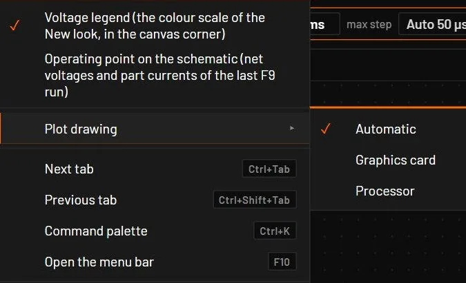
The Analysis plot draws its traces on the graphics card (WebGL2), up to 144 frames a second with 100 traces, from the same minimum and maximum of each pixel column as before, so the picture does not change. picks Automatic (the default: the graphics card where it works), Graphics card or Processor. Where the card is missing or fails, the processor draws the plot. A big run also needs about 40 % less memory on its way to the plot: its columns are sized up front, and the desktop app sends big pieces compressed when that is faster on the machine.
29.9Working with the plot
| Action | How |
|---|---|
| Read values | Hold the pointer over the plot. A line follows the pointer and a box lists every trace at that point, up to 16. |
| Zoom | Drag a box. A box taller than 12 px also zooms that pane vertically. The wheel zooms in time around the mouse. Neighbouring ticks never read the same (see below). |
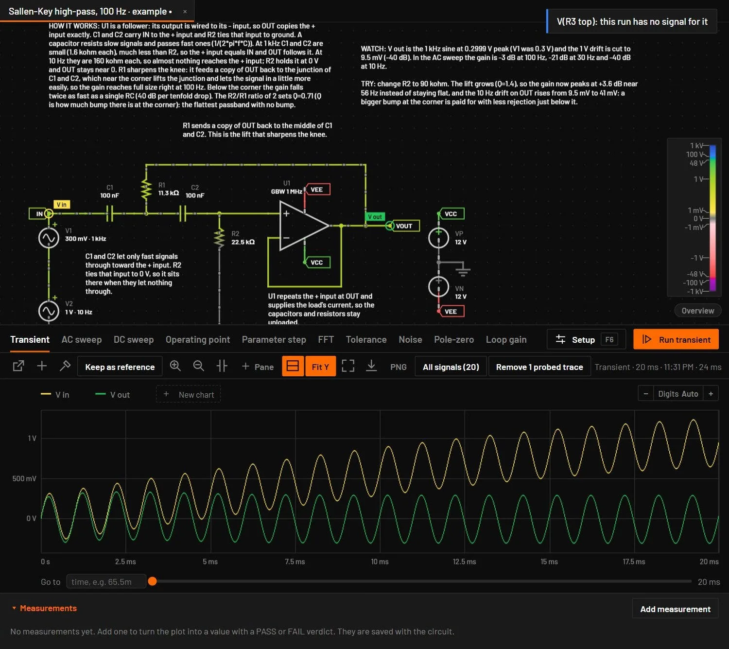
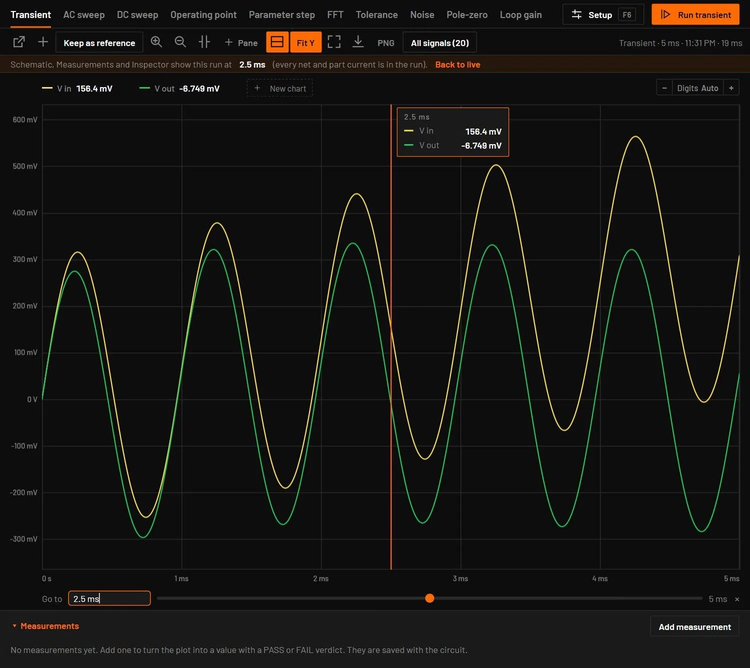
| Go to a time | The Go to bar below a transient plot: type a time such as 65.5m and press Enter, or drag the slider through the run (zoomed in, it moves at the scale of the plot). An orange playhead marks the time with a box of the value of every trace there. When you're zoomed in, the view centres on it and keeps the zoom. Drag the playhead line to move it, and click × to remove it. |
| Pan | Ctrl-drag, Shift-drag, right-drag or middle-drag. |
| Reset | Double-click. |
| Find a trace on the schematic | Hold the pointer over its name in the legend. The net or part lights up on the canvas. |
| Add a trace | In Split view, Alt+click a net for its voltage or a two-pin part for its current. A plain click selects and edits as in the Schematic view. If the last run kept only the probes, it reruns with the new trace and says so. |
29.10Axis labels and readout digits
Every plot (the Analysis view, Split, pop-outs, the live scope, Bode and FFT) writes its ticks so that no two read the same. An ordinary axis looks as it always did. When a label would need more than 6 significant digits or would not fit the axis, as with a 0.2 nV ripple on 15 V, the base is written once, in bold, in the corner of the pane (15.0579 V +) and the ticks show the offset from it (+88 µV to +98 µV). The time axis does the same when you zoom far in: 86.5933 µs + at the left of the labels, then +90 ps to +130 ps. dB and degree axes get more decimals, or an offset with one exponent far below one.
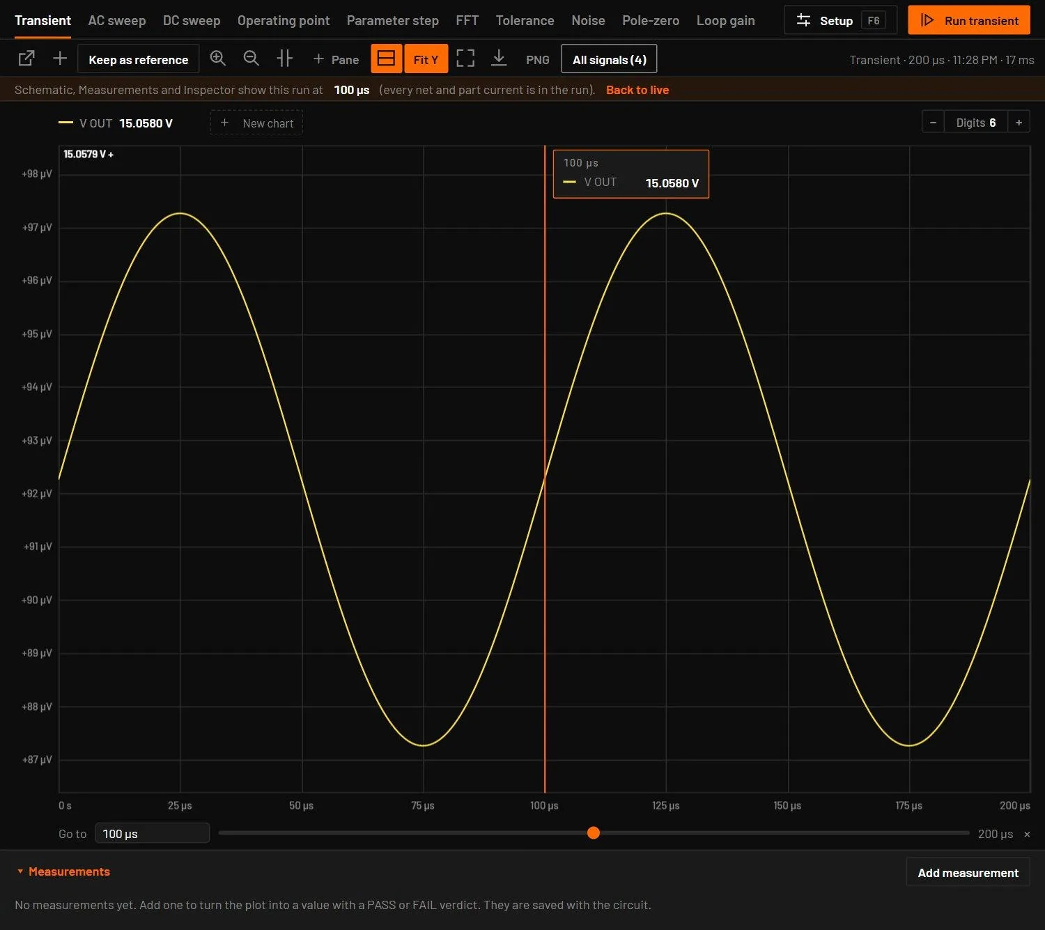
− Digits Auto + at the right end of the legend strip (also in Split and the pop-out) and in each live scope's header sets how many significant digits the readouts show, from 3 to 9:
- − and + step it, the mouse wheel over it steps too, and a click on the number goes back to Auto. Auto keeps the look of earlier versions: 4 digits in tooltips and chips, 3 in tables.
- One setting serves the Analysis view and every scope, so a value read in two places shows the same digits. It is remembered.
- It covers the hover tooltip, the playhead values, the cursor table, the trace chips, the signal list, the statistics, the operating point table and Measurements.
- A number keeps its trailing zeros, so a readout keeps its width while the value moves: 15.0580 V at 6 digits, where Auto reads 15.06 V.
- It changes only what is shown. CSV export and Copy as table write every digit. Time readouts already follow the zoom and keep their own digits.
Traces cycle through yellow, green, orange, blue, violet and red. The vertical range fits the visible data with a small margin. A footnote lists probes the run has no signal for, for example an AC current through a part that has none.