
Live simulation
The live simulation starts when a circuit opens and runs while you edit. The status bar says running or paused. Every frame it solves the circuit's equations for the next stretch of circuit time and redraws the colours, dots and readings.
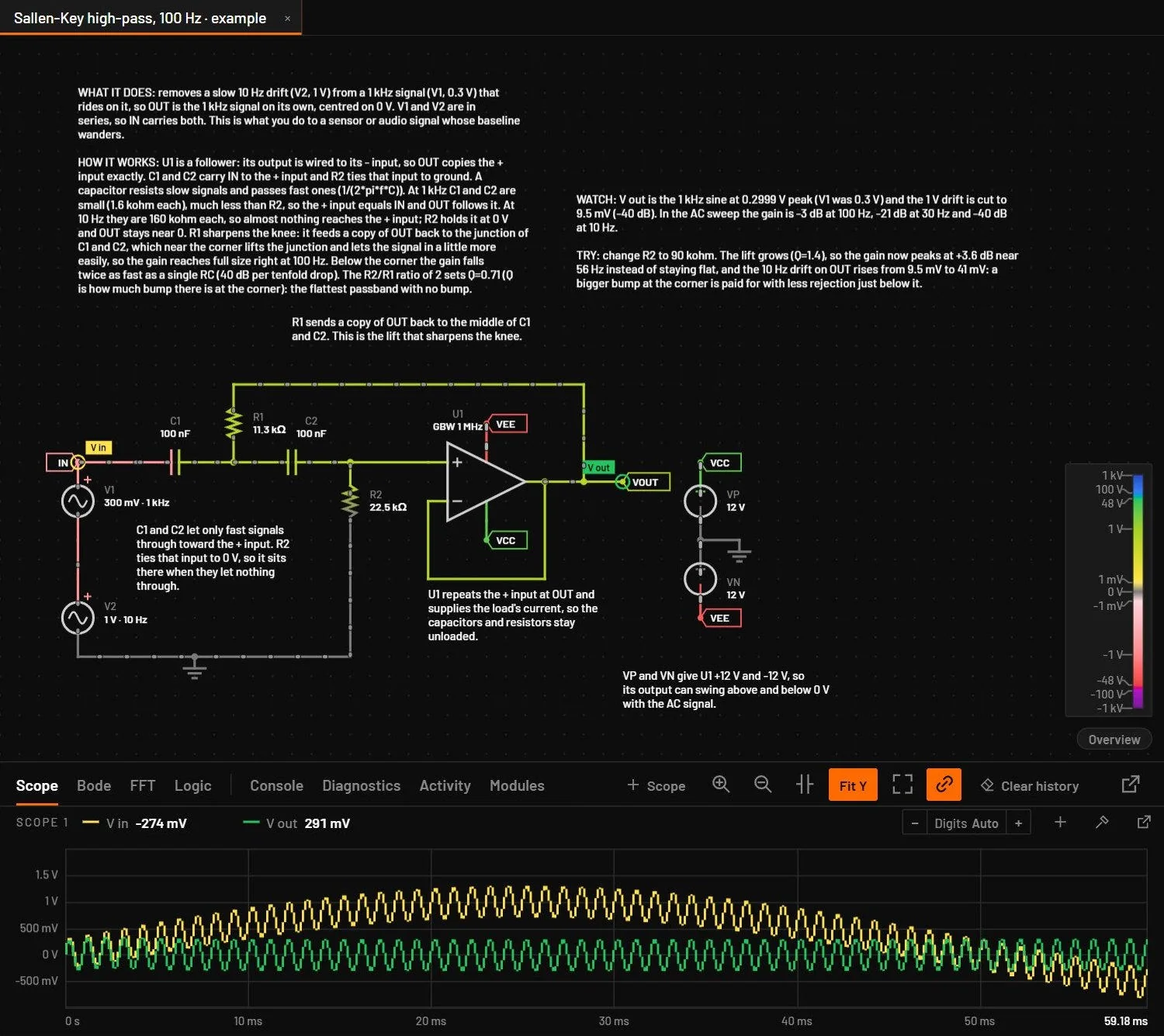
25.1Run, pause, step and reset
| Control | Key | What it does |
|---|---|---|
| Run / Pause | Ctrl+R | Starts or pauses the live simulation (the browser viewer keeps Space for this). Holding Space and dragging pans. |
| Step | . | Advances by one timestep. Pause first to see one step at a time. |
| Reset | Ctrl+Shift+Backspace | Restarts at t = 0 from the circuit's start state (below), with counters cleared. |
| Sim time | toolbar | The simulated time since the last reset, four digits with a prefix. |
25.2Start at rest or from the operating point
The live simulation can start in two ways. At rest (power-on): every node at 0 V, capacitors empty, inductors without current. A first RC filter then visibly charges. From the operating point: the circuit starts already settled, as if it had been running for a long time, the way a regulator example opens at its output voltage.
| Circuit | Starts |
|---|---|
| Made with (or a new tab) | At rest. |
| An example, or a file saved before this option | From the operating point. |
| A circuit where a capacitor or inductor has an Initial voltage or Initial current | From those values, as ic does in SPICE. Setting any initial value, even 0, makes the whole live start use initial conditions. |
shows a tick when the open circuit starts at rest. Choose it to switch, and the simulation restarts from t = 0. The choice is saved in the circuit file. Reset (above) starts again the same way. It applies to the live simulation only: Simulate starts from the operating point unless the circuit asks for initial conditions (Settings saved in the circuit).
Initial voltage and Initial current are in the part's full parameter list (All N parameters in the inspector).
25.3Timebase and speed
The timebase sets how much simulated time passes per real second. A 50 Hz mains waveform is unreadable at real time on a screen, but at 10 ms per second one cycle takes two real seconds.
| Field | Values | Default | What it does |
|---|---|---|---|
| Timebase slider | 1 to 1000 of the chosen unit, per second | from the circuit, else 10 ms/s | Drags within the chosen unit and snaps to 1, 2 and 5 near each decade. A drag past the right end rolls on into the next unit (1000 ns, then 1.1 µs and on), past the left end into the one before. |
| Timebase field | a number, or a number with a unit | 20 means 20 of the chosen unit. 20n, 20 ns, 1e-8 and 2m are absolute and switch the unit. Enter applies, Esc cancels. | |
| Unit | ps, ns, µs, ms, s | A new unit lands next to the old value: a unit up starts at 1 of it, a unit down at 1000 of it. | |
| Range | 1 ps/s to 10 s/s | Slower than 1 ps/s or faster than 10 s/s is clamped. |
| Key | Speed preset | Good for |
|---|---|---|
| 1 | 1/1000: 1 ms per second | Switching converters, PWM, oscillators in the kHz range |
| 2 | 1/100: 10 ms per second | Mains rectifiers, audio |
| 3 | 1/10: 100 ms per second | RC charging, slow filters |
| 4 | 1x: real time | Thermal and battery circuits, relays, motors |
The live engine also has a timestep, shown in the toolbar and status bar. It's set per circuit (1 µs for a new circuit) and kept small enough for the circuit's fastest events. When the computer can't keep up, simulated time runs slower than the timebase rather than becoming inaccurate.
The scope shows the last 6 real seconds, so a fast timebase puts many cycles on screen. At 12 ms/s a 13 kHz oscillator fills the window with about 900 cycles, and the scope draws them as a solid band between each trace's lowest and highest value, as an oscilloscope does. Zoom in with the wheel while it runs: like shortening an oscilloscope's time per division, a zoomed view makes the scope sample faster, and each cycle keeps its real shape at any timebase. Zoomed out, the scope keeps only a few points per screen pixel, so a fast timebase doesn't load the computer. Detail is captured only while you're zoomed in: zoom in before you pause to inspect cycles, because data recorded while zoomed out stays coarse. The part of the window older than two zoomed views is dropped and fills in again when you zoom out.
25.4Live quality
The menu after the timebase unit sets what the live view may give up to keep the timebase. Simulate (F5) never changes with it.
| Setting | What the live view does |
|---|---|
| Exact (the default, every session) | Runs the circuit as drawn, at its own step. When this computer cannot run it at the timebase, the view runs slower. The toolbar shows the real speed in amber, for example runs at 162 µs/s, and a banner over the schematic says why, with Balanced and Fast buttons. A circuit with fast sources or a short sim.dt can be far slower than the timebase: a 6 MHz sine needs 20 steps a cycle. |
| Balanced | Keeps the timebase by raising the live step above the circuit's own, to at most a 200th of the timebase. Edges, ringing and MHz ripple are drawn coarser. |
| Fast | As Balanced, and every sine source faster than 1000 divided by the timebase (1 MHz at 1 ms/s, 1 kHz at 1 s/s) is held at its average. Each one is named in the banner, tagged Averaged in live view on the schematic and listed in Diagnostics. |
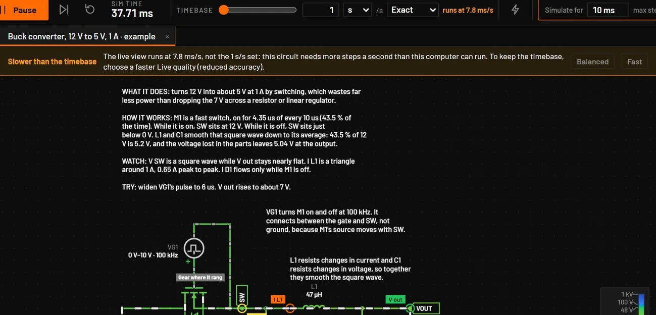
While Balanced or Fast changes anything, the banner says Reduced accuracy and names what is changed, and it offers Back to Exact. A switching circuit whose edges set the step (PWM) can still run slower than the timebase in Fast. The banner then says so too.
25.5Changing the circuit while it runs
- Changing a value, by typing or with a slider, applies at once and keeps the circuit's state. Turn a potentiometer and watch a capacitor charge to the new level. Change a capacitor's value and it keeps its voltage, change an inductor's value and it keeps its current, and a diode's capacitance changes the same way. Before 0.7.0 the node voltage jumped to a different value at the edit. Simulate always starts from the beginning of the run.
- Adding, deleting or rewiring parts also keeps the state of the parts that stay. A relay keeps its contacts as they were.
- A value you set while it runs (typed or picked, not dragged) starts the live step again from first order, as a fresh run would, so the next steps are as accurate as Simulate's. A frequency or period you change becomes that source's step limit at once, and a value that rebuilds the part, such as a capacitor's ESR, keeps the step the timebase and Live quality set. A dragged slider keeps its step.
- Clicking a switch toggles it. Push buttons stay pressed while the mouse button is down.
- An LED glows in proportion to its current: visible from 0.5 mA, with a solid lit body, a pale core and a wide soft halo that is full size at its rated current. Relays, switches and potentiometers draw their state.
- Readings are cleaned of numerical noise. A voltage, current or power below a billionth of the circuit's own scale reads 0 in the inspector, Measurements, the scope legend and the hover card. The exact value is in the tooltip, and exported CSV and copied data keep the raw numbers.
25.6Several circuits at once
Each open circuit tab keeps its own live simulation. When you switch away, BetterSPICE parks it with its traces, scope history, logic recordings, timebase, diagnostics, and its running or paused state, and picks it up when you come back: a rectifier that was paused at 150 ms is still paused at 150 ms. BetterSPICE keeps up to four background tabs. Beyond that a tab restarts from t = 0. A circuit you open fresh always runs. While the Analysis view fills the whole window, the live view redraws about four times a second instead of sixty to save work. The engine keeps running and the scope keeps every sample.
25.7Current dots
Dots move along wires and through parts in the direction of conventional current. They are display only. How they look depends on the live look (below). In the New look the dots grow with the current, from a small faint dot at 1 µA to a long bright dash at 20 A, always 28 pixels apart. Their speed is nearly even up to about 1 A (50 pixels a second at 1 µA, 107 at 1 A) and only gets clearly faster for large currents (387 at 10 A). A dot never moves so far in one frame that it seems to run backwards. In the Classic look the dots are yellow, of one size, and their speed follows the square root of the current.
| Control | Key | What it does |
|---|---|---|
| Current slider | toolbar | Dot speed from 0.01x to 100x. It snaps to 1x in the middle. Double-click for 1x. |
| Faster / slower | ] / [ | x1.5 or /1.5 per press, beyond the slider's range if needed. |
| Fit | Shift+] or Fit | Sets the speed so the largest current in the selection, or in the whole circuit, moves about 150 pixels per second, by the speed rule of the live look in use. Select a part first to study its current. |
| Reset | View menu | Back to 1x. |
If Windows is set to reduce motion, the wires show fixed arrows for the current direction instead of moving dots.
25.8Energy view
Alt+E, the lightning bolt in the toolbar, or shows where the power of the running circuit comes from and where it goes. It is off when the app starts and it replaces the current dots while it is on. With it off, the canvas costs what it did before.
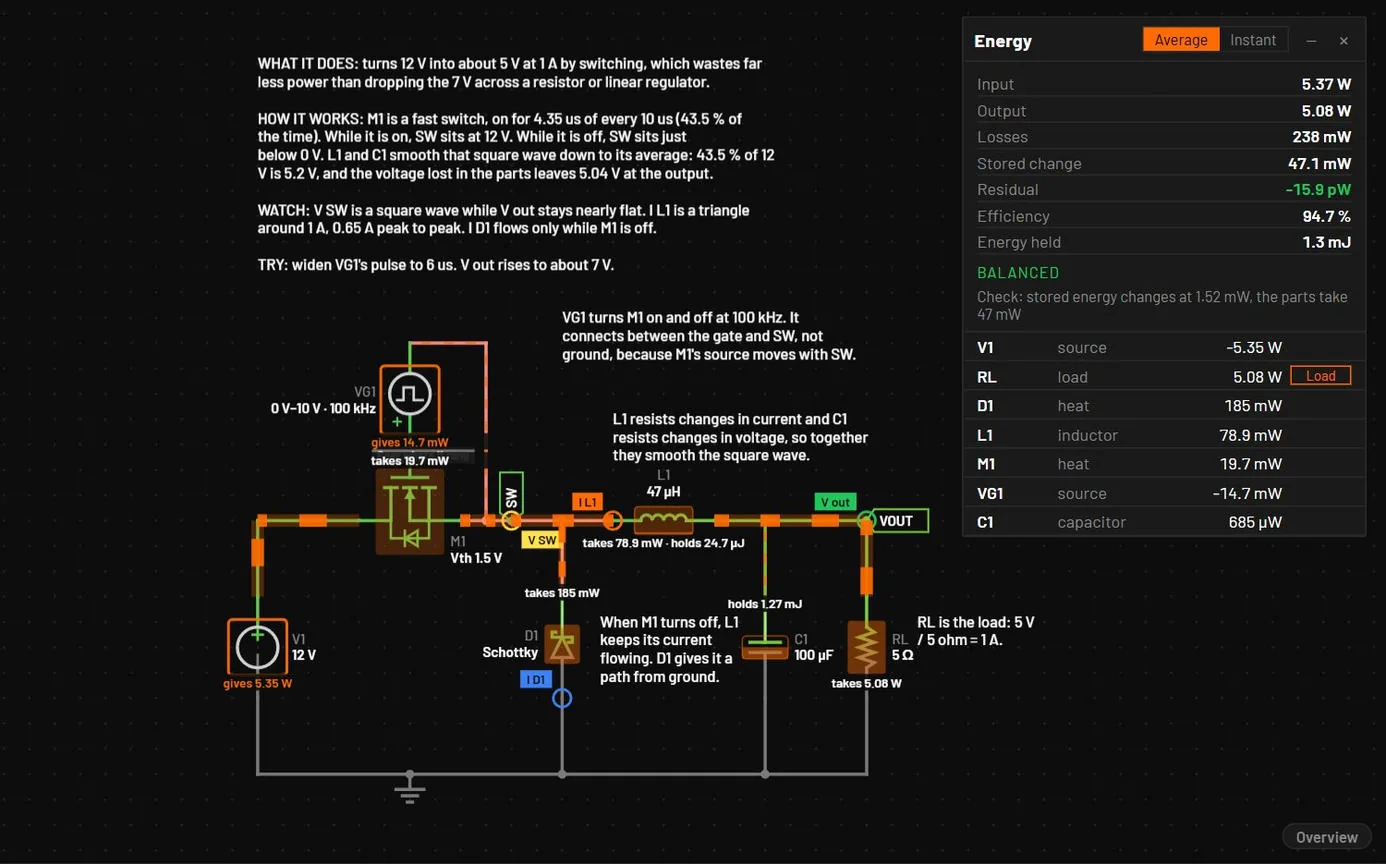
| What you see | What it means |
|---|---|
| Flow bands | A band lies on every wire that carries power. Its width grows with the power on a log scale (the thinnest band is a thousandth of the widest). Its dashes move from the end the power comes from to the end it goes to. The power on a wire is its voltage to ground times its current. With reduced motion set, an arrowhead replaces the moving dashes. |
| Parts that give power | An orange outline and the words gives 5.8 W. A part that takes power says takes. |
| Parts that make heat | An orange wash that deepens with the loss. |
| Capacitors and inductors | A level that rises with the energy held (½CV² or ½LI²) against the part's own largest value of the last 30 seconds, and the words holds 26 µJ. |
| Ledger | A panel with Input (net power of the sources), Output (the loads), Losses (including capacitor ESR and inductor DCR), Stored change, Efficiency and Energy held. Residual is input minus output, losses and stored change. It is zero when every pin current is accounted for, and the panel says Does not balance in red when it is not. Click a row to select the part. |
- The ledger stands in a corner where it covers no part, label or note. When the circuit leaves no room, it opens folded to its header, which shows the input power and the efficiency. The plus button unfolds it.
- Average is a moving average over about half a second of wall time, so a switching circuit reads steadily. Instant shows each frame as it is, ripple included.
- The load is an LED, lamp, motor, speaker or buzzer, or a resistor named RL, RLOAD or LOAD. The Load button on a resistor's row changes that for the session. A part parameter
loadset to true or false is saved with the circuit. Without a load there is no efficiency. - A switching circuit can have edges faster than the engine's steps. The moving average then cannot split the loss between the parts. The ledger tests for this, and when a test fails the panel says Not measurable at this timebase with the reason and shows no losses or efficiency. A slower timebase or Instant still works. The flyback example is such a case.
- The power on a wire is relative to ground. Transformers and chokes show the power they take as stored change, because their stored energy is not modelled.
25.9Tolerance band
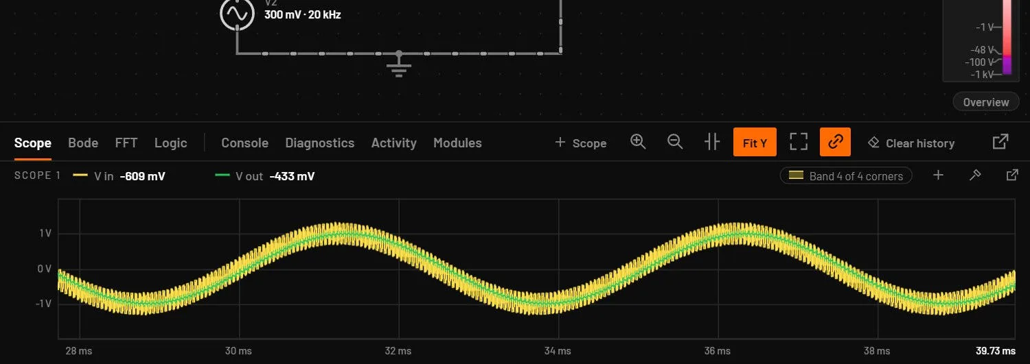
(also in the scope menu under Display, off by default) shades, around each scope trace, the range it takes with the parts at the ends of their tolerance: resistors 1 %, capacitors 10 % and inductors 20 % unless a part says otherwise. Extra live engines, one per corner and each in its own worker, follow every edit and the timebase and never run ahead of the trace. Every corner runs when they fit (up to 8, or 16 with every corner), otherwise the two extremes, and the label in the scope header says which, for example Band 4 of 4 corners. The corners are those bspice app tolerance --mode worst picks, and the trace itself does not change. The band stays off, with its reason in the label, with Balanced or Fast quality, while the MCU debugger is used, or when the machine has too few free workers or memory.
25.10Heavy circuits
In the desktop app a circuit with 100 parts or more runs the live view on the native engine, about 1.4x as fast as WebAssembly on a 578-part board, with the same frames bit for bit. The status bar then reads Live MNA · native. Smaller circuits, the browser viewer and a board with the tolerance band on stay on WebAssembly.

25.11Energy view and the scope history
With the run paused, move the scope's playhead back through the history and Energy view shows that moment: its figures and colours follow the playhead, like the wires. Clear the playhead to go back to live.
25.12Drawing
The schematic is drawn again only when something on it changes (a value, the view, an edit), and the current dots and wire colours draw on the graphics card where it can, with the processor as the fallback.
25.13Live look
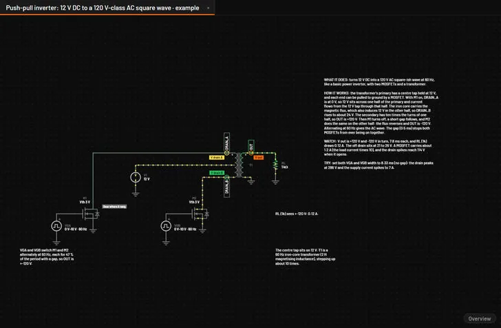
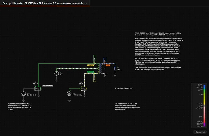
has two entries, New and Classic. New is the default, also on a copy that was updated. The look you pick here is remembered.
| New | Classic | |
|---|---|---|
| Wire colour | One absolute scale, so the same voltage always has the same colour, in every circuit. A lighter wire always means a smaller voltage. | Stretched to the circuit's voltage range, 10 V unless the circuit file sets another. |
| Positive voltage | Pale yellow at 1 mV, through lime, to green at 48 V. Then through teal to blue at 100 V, and deeper blue up to 1 kV, so anything past the 50 V safety mark reads at once. | Green, or orange with the orange and blue colours. |
| Negative voltage | Red only: pale rose, red at -48 V, then crimson and purple at -100 V. | Red, or blue with the orange and blue colours. |
| Near 0 V | Neutral grey. Noise such as a nanovolt stays grey, and the colour blends in smoothly up to 1 mV. | Neutral grey. |
| Current dots | Size and brightness show the current (above). | Yellow, of one size. |
| Colour choice | Ctrl+Shift+K is greyed out and says that voltage colours belong to the Classic look. | Ctrl+Shift+K switches between green and red and orange and blue. |
The light theme keeps the same order of colours and keeps them readable on a light background. The New look draws as fast as Classic.
25.14Voltage legend
In the New look a slim bar in the bottom-right corner of the schematic shows the colour scale: +1 kV at the top, 0 V grey in the middle, -1 kV at the bottom, log in decades, labelled at 1 mV, 1 V, 48 V, 100 V and 1 kV and their negatives. Hold the pointer over a wire, pin or net label and its voltage is marked on the bar with its value. The legend moves left of the sheet overview when that is open and never takes a click. hides it, and the choice is remembered. The Classic look has no legend.
25.15Hover readouts
| Pointer over | The card shows |
|---|---|
| A wire | The name and voltage of the net, and the current in that wire. |
| A net label, power flag or port | The name and voltage of the net. |
| A pin | The part and pin, the voltage of the pin, the current into it and the power of the part. A pin is also where a drag draws a wire, and the card says so. |
| A part | V, I and P of the part, and for a part with more pins the voltage and current of each pin. |
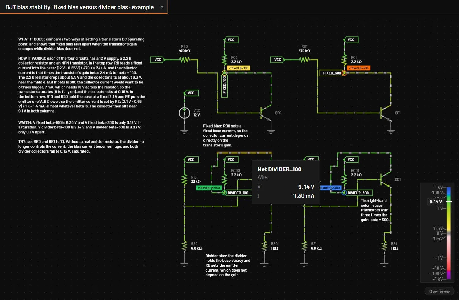
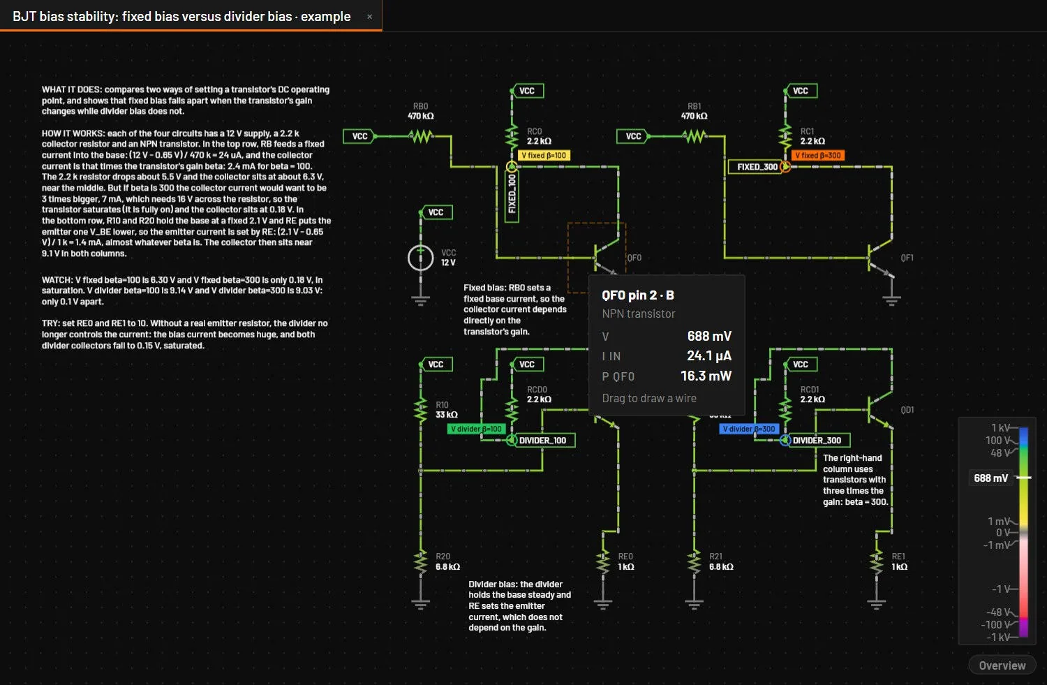
The values are the ones the inspector shows, at its update rate (Update in Measurements) while the circuit runs. Paused, they are the paused moment, or the moment under the scope's playhead. The card never takes a click, and it is off while you drag, draw a wire or place a part.
25.16Voltage colours
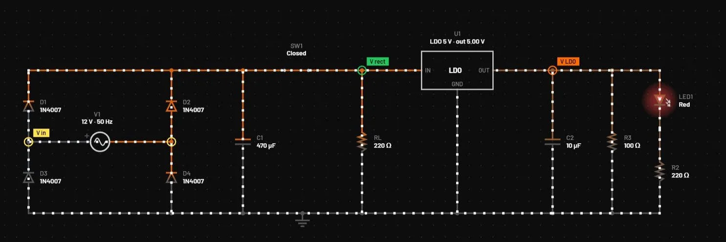
In the Classic look, wire colour goes from the zero colour at 0 V to the full positive or negative colour at the circuit's voltage range, 10 V unless the circuit file sets another. Ctrl+Shift+K, or , switches between the default green and red scale and the orange and blue scale. In the New look this entry is greyed out, because that look has one scale for every circuit.
25.17Halted
When the engine can't continue, for example because a node has no DC path to ground, it stops. The Run button turns into a red Halted button, the canvas shows Halted · code, and the Diagnostics tab lists the reason with the part, the net and the fix (Diagnostics and what they mean). Fix the circuit and the simulation starts again.
25.18Live MNA · JS
What you see: the status bar says Live MNA · JS and the live simulation runs slower than usual. Cause: the WebAssembly engine could not load (an E_ENGINE warning says why), so the live view runs on the JavaScript engine. Fix: none is needed, and a restart usually brings the WebAssembly engine back. From 0.8.0 the JavaScript engine runs every part type the main engine has, microcontrollers and their programs, ctrl scripts, logic packages, motors and converters included, on the same device equations. It solves the operating point when the circuit loads, finds switching edges and breakpoints, and sizes its steps by the truncation error, as the main engine does. A part that no engine can simulate is left out of the run with a W_SYMBOL_ONLY warning, and the rest of the circuit keeps running.
25.19How the live engine works
The live engine is a circuit solver, not an animation. It writes the circuit as equations by modified nodal analysis (MNA), turns capacitors and inductors into companion models for each timestep, and solves the nonlinear parts by Newton iteration. It's compiled to WebAssembly so it keeps up with your edits.
It is the engine Simulate uses, and the two agree: the first live step is exactly the first step of Simulate, and at the same step the live view reproduces Simulate bit for bit. The live view always steps with the trapezoidal rule and gmin 1 pS. When the Simulation setup asks for Gear or another gmin, a W_LIVE_SETUP note says so, and Simulate uses the setup.
A vendor subcircuit runs in Simulate. In the live view it runs on its fitted stand-in where it has one: the four UC3843 examples run live on the uc384x controller with a TL431 and an opto fitted to the vendor models, and are checked against the vendor models in Simulate. A vendor part with no stand-in, such as TI's averaged PWM models, has its pins open in the live view, and its message says it is accurate-only.