
Analyses and their setup fields
The Analysis menu runs the classic SPICE analyses. F6 opens Simulation setup, with one tab per analysis, an explanation beside every field, and a Run button. The setup is saved in the circuit file.
28.1The setup dialog
- Tabs: Transient, AC sweep, DC sweep, Operating point, Parameter step, FFT, Tolerance, Noise, Pole-zero and Loop gain. The last three are in the Analysis menu and have no function key.
- Values read from the circuit show in engineering notation (
1G,1µ,1.59155k, up to six digits so nothing is lost on save), and the fields read them back. - Number fields check what you type as you type. Text that's not a number turns red with "Not a number. Use plain values or SI prefixes such as 200m, 1u, 10k, 1Meg." and disables Run.
- The dialog puts the focus in its first field and keeps Tab inside. Enter anywhere runs, also from a number field. Reset tab restores that tab's defaults. Close (or Esc) keeps your changes without running.
- Run closes the dialog and runs, and the result shows as for every run: from the Schematic view the window splits. In Split and Analysis it stays.
- A new circuit fills the setup from its own parts: the AC and DC sources are real sources of the circuit, the step parameter is its first resistor, the FFT signal its first probe.
- Source, output node, parameter and probe fields list what the circuit has to choose from, and say when a name you typed isn't in it. A current source's DC sweep is in amperes.
- The source, output-node and probe fields have a pick on schematic button: the dialog closes, you click the source, net or probe on the canvas, and it opens again with the field filled. Esc cancels. Clicking something that doesn't fit says why.
- The settings of every tab are saved in the circuit file, as an undoable edit that marks the circuit changed, and a circuit reopens on the analysis it showed last. Running an analysis doesn't mark the circuit changed and isn't an undo step.
The analysis keys. Shift+F5 (transient), F7 (AC), F8 (DC), Shift+F7 (step) and Shift+F8 (FFT) run that analysis with the setup saved in the circuit. The first time, when the circuit has no setup for it, the key opens the setup instead, and Run there saves it, so the key runs it from then on. The setup header says so: F7 runs it from now on · F6 opens this setup. F6 opens the setup of the current analysis at any time, and the toolbar's .ac and .step buttons open theirs. F9 runs the operating point at once. F5 runs a transient with the toolbar's stop time and max step.
| Analysis | Key | Result |
|---|---|---|
| Transient | Shift+F5, or F5 to run it directly | Signals against time |
| AC sweep | F7 | Gain and phase against frequency, with -3 dB points and margins |
| DC sweep | F8 | Signals against a swept source value |
| Operating point | F9 runs it at once | A table of node voltages and branch currents |
| Parameter step | Shift+F7 | One curve per parameter value, overlaid |
| FFT | Shift+F8 | A spectrum in dB against frequency |
| Tolerance | Shift+F9 | Monte Carlo or worst case on the part tolerances |
| Noise | Analysis menu | Noise density at an output, each part’s share, and the totals |
| Pole-zero | Analysis menu | Poles and zeros of a transfer function, on the s-plane and in a table |
| Loop gain | Analysis menu | Bode plot of a feedback loop with the crossover, phase margin and gain margin |
28.2Transient
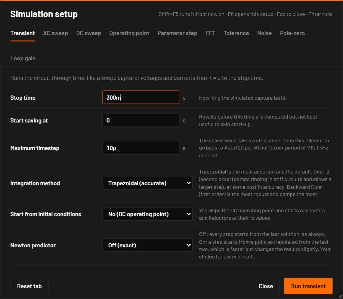
Runs the circuit through time, like a scope capture: voltages and currents from t = 0 to the stop time.
| Field | Values | Default | What it does |
|---|---|---|---|
| Stop time | seconds, above 0 | 200m | How long the simulated capture is. Also the Simulate for field in the toolbar. |
| Start saving at | seconds, 0 or more | 0 | Results before this time are computed but not kept, to skip the start-up. It must be earlier than the stop time: otherwise the field says "Must be earlier than the stop time…" and Run is greyed. |
| Maximum timestep | seconds, above 0, or empty or auto | Auto | The solver never takes a longer step. Smaller is more precise and slower. Empty means Auto: the step is chosen from the circuit (Auto maximum step). Also the max step field in the toolbar. |
| Integration method | Trapezoidal (accurate), Gear-2 (damps ringing), Backward Euler (most robust) | Trapezoidal | Trapezoidal keeps the most detail. Gear-2 (second order) damps ringing in stiff circuits and allows a larger step, at some cost in accuracy. Backward Euler (first order) is the most robust and damps the most. Used by ngspice runs and by the BetterSPICE engine. Choose a damped method when the run warns W_TRAP_RINGING (a numerical oscillation of the trapezoidal rule, explained in the Fix chapter). |
| Start from initial conditions | No (DC operating point), Yes (ic values) | No (DC operating point) | Yes skips the DC operating point and starts capacitors and inductors at their ic values. Used by ngspice runs. The BetterSPICE engine starts from ic values when the circuit sets them. A circuit can set this, the method and ngspice options itself (Settings saved in the circuit). |
- Open Switching converters, a synchronous buck.
- Press Shift+F5. Set Stop time
2mand Maximum timestep50n. Press Enter.
You should seeThe output rises to its set voltage with the soft start, and the inductor current shows the ripple. Zoom into the end to read the steady ripple.
28.3AC sweep
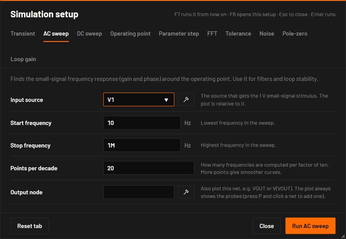
Finds the small-signal frequency response, gain and phase, around the operating point. The circuit is linearised at its DC operating point, the input source gets a 1 V small-signal stimulus, and every probe is plotted relative to it.
| Field | Values | Default | What it does |
|---|---|---|---|
| Input source | a source designator | the circuit's first source | The source that gets the 1 V stimulus. An unknown name is refused with the list of the circuit's sources. |
| Start frequency | Hz | 1 | The lowest frequency. |
| Stop frequency | Hz | 1Meg | The highest frequency. |
| Points per decade | number, at least 1 | 50 | Frequencies per decade. |
| Output node | a net name, optional | empty | Also plot this net, written VOUT or V(VOUT). Probes are always plotted. |
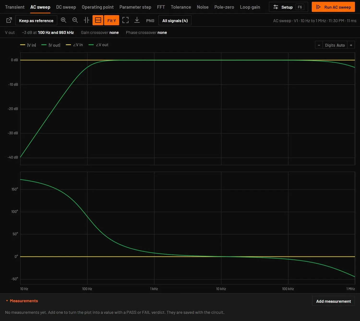
The result is a Bode plot: magnitude in dB and phase in degrees. Where the gain is below −200 dB the phase isn't drawn, and when every probe sits at that floor the result says "No small-signal path from V1 to … at this operating point". The phase is unwrapped, so it runs on past −180° without jumping by 360°, in the plot and in bode.csv. The margins strip above it shows, for the output trace, the -3 dB frequencies (up to two), the Gain crossover, the Phase margin (amber below 45°), the Phase crossover and the Gain margin (amber below 6 dB).
28.4DC sweep
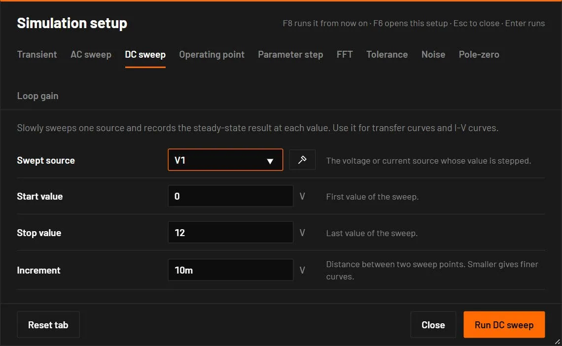
Slowly sweeps one source and records the steady-state result at each value.
| Field | Values | Default | What it does |
|---|---|---|---|
| Swept source | a DC voltage or current source | the circuit's first source | A battery can't be swept. The message suggests a DC voltage or current source instead. |
| Start value | V or A | 0 | The first value. |
| Stop value | V or A | twice the source's value | The last value. For a 300 mV source the default sweep is 0 to 600 mV. |
| Increment | V or A | about 1/500 of the range | The step between values (1 mV for a 300 mV source). |
The caption of the result carries units, for example V1 0 V to 600 mV.
- Place a DC source, a 100 Ω resistor and a diode in series, and probe the current through the diode.
- Press F8. Sweep the source from
0to2in5msteps.
You should seeThe current stays near zero until about 0.6 V across the diode, then rises steeply, limited by the resistor.
28.5Operating point
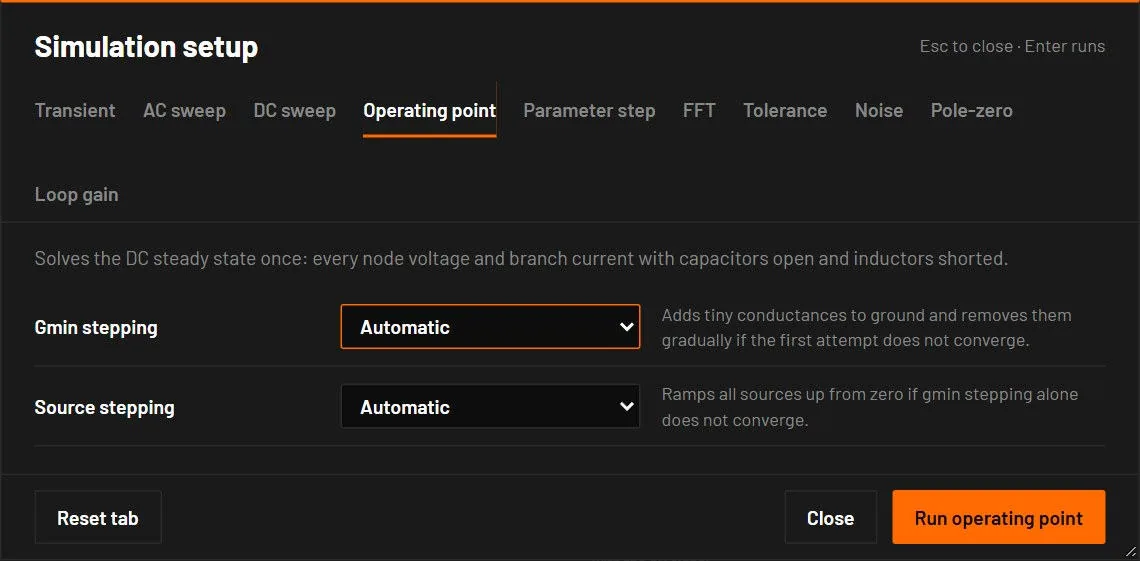
Solves the DC steady state once. F9 runs it at once without the dialog.
| Field | Values | Default | What it does |
|---|---|---|---|
| Gmin stepping | Automatic, Off | Automatic | If the first attempt fails, adds tiny conductances to ground and removes them step by step. |
| Source stepping | Automatic, Off | Automatic | If gmin stepping fails too, ramps the sources up from zero. |
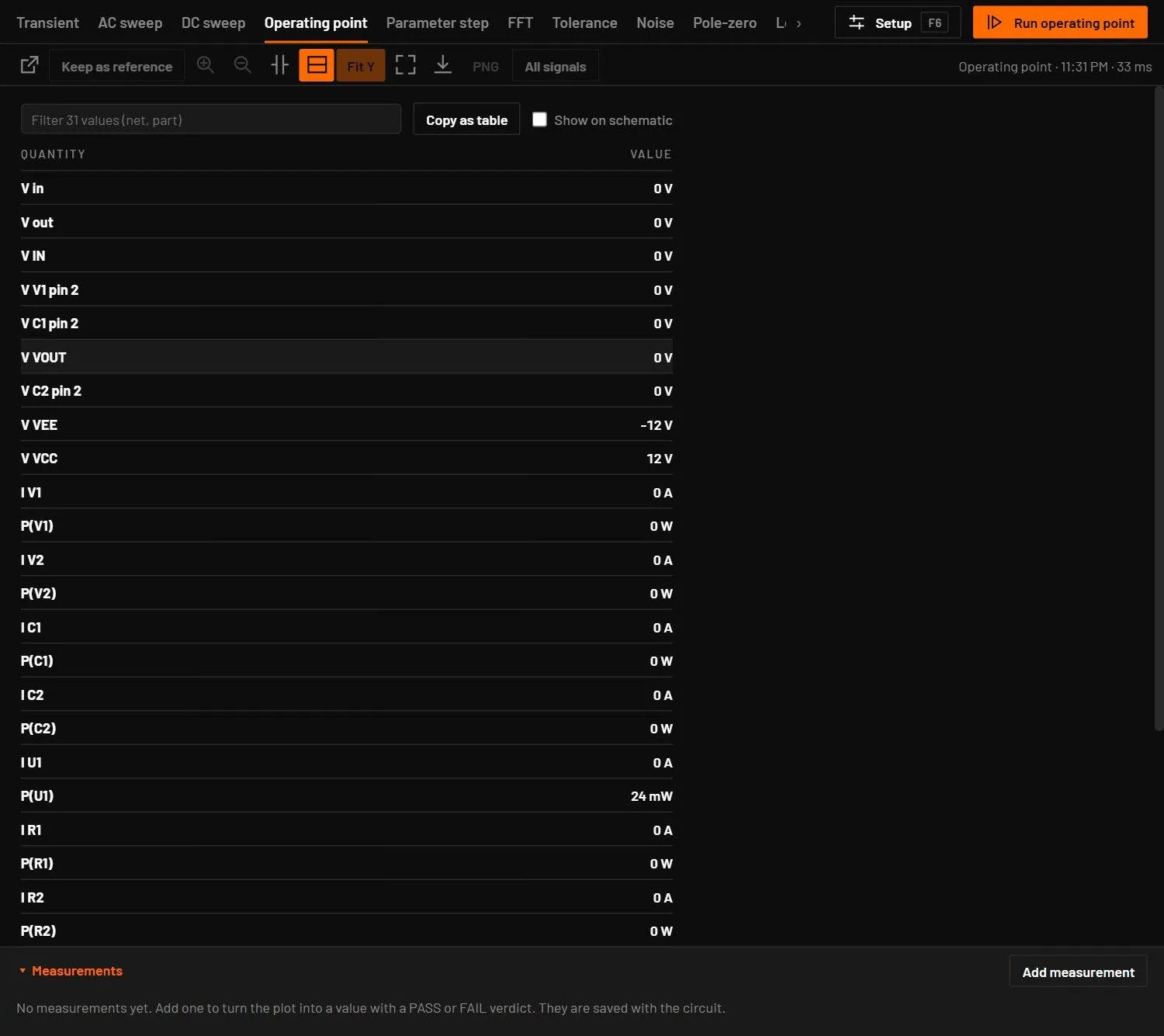
Off only applies to ngspice runs. The BetterSPICE engine uses both when it needs them and says so. The result is a table: probes first, then V(net) for every net, then I(part) and, for runs in the BetterSPICE engine, P(part). Nets are named as on the schematic: a label, else a part pin such as V(C1 pin 2). Click a row to mark its net or part on the schematic. With more than 12 rows a filter box appears, and 300 rows show until Show all. Copy as table puts the table on the clipboard. Export CSV writes Quantity, Value and Unit.
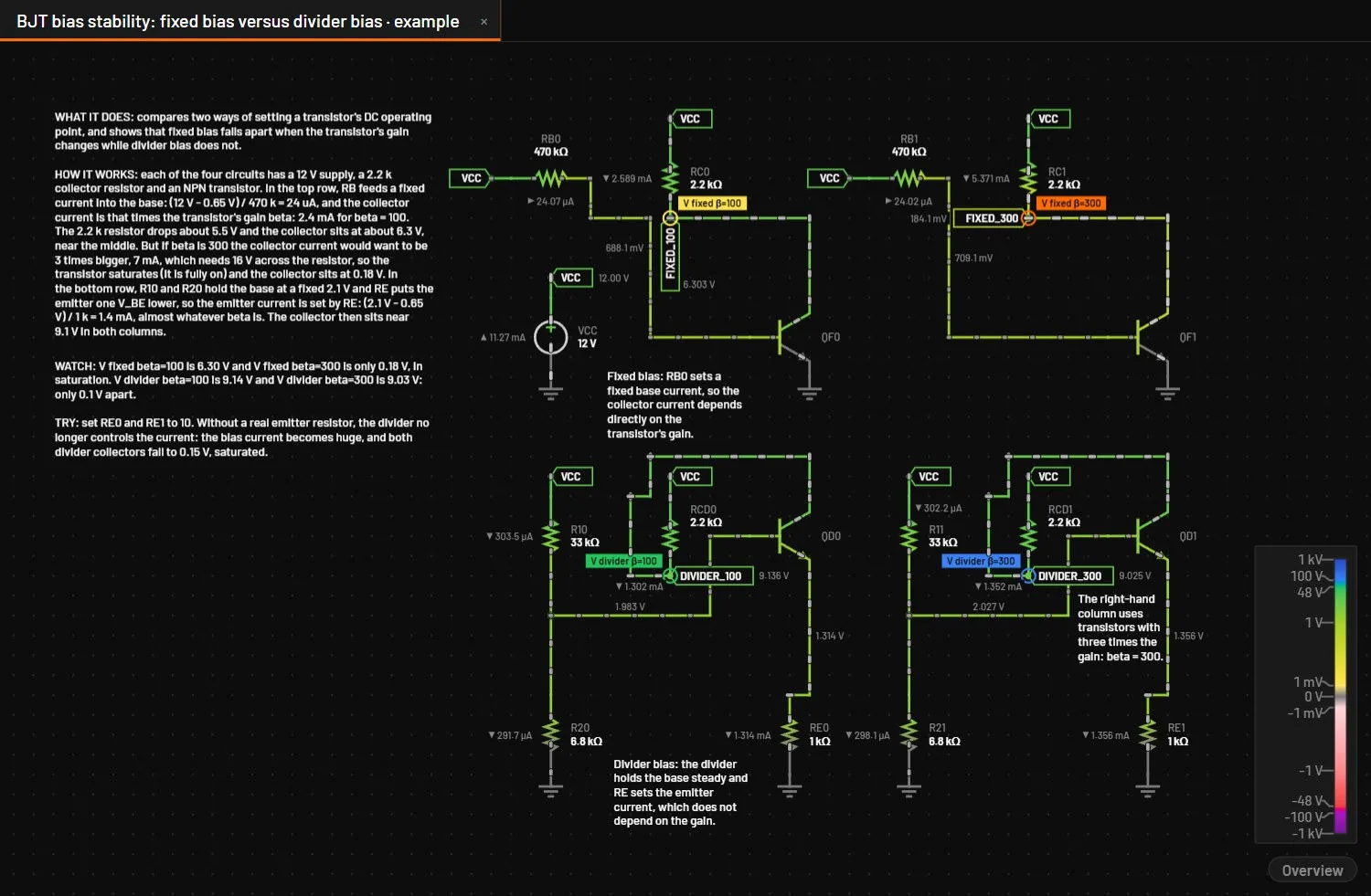
Show on schematic above the table (or ) writes the result on the circuit: every net's DC voltage (ground left out) beside its net label or along one of its wires, and the current of every two-pin part that carries DC current, with a small arrow in the direction it flows through the part. A capacitor carries none and gets no label. The text is small and muted, the numbers are those of the table, and each one is placed clear of parts, labels, probe tags and the other values. When there is no room for one, it is left out: zoom in, or read it in the table. The values go away as soon as the circuit changes and come back with the next F9. The switch is remembered.
28.6Parameter step
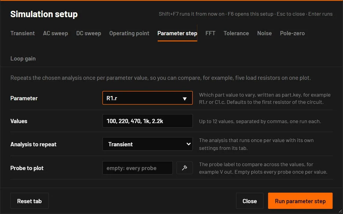
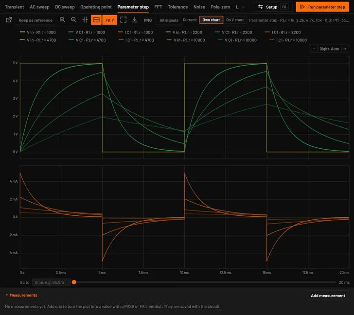
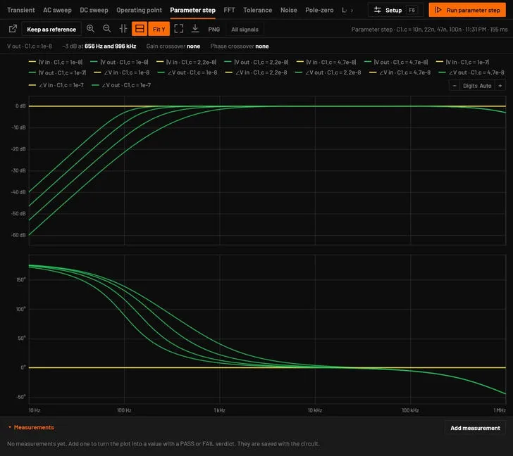
Repeats the chosen analysis once per parameter value and overlays the results.
| Field | Values | Default | What it does |
|---|---|---|---|
| Parameter | part.key | the first resistor, R1.r | The value to step, written as the designator, a point and the parameter key: R1.r, C1.c, V1.v. The keys are in the parameter tables of the device chapters, from Devices: passives on. |
| Values | a comma list, at most 12 | 100, 220, 470, 1k, 2.2k | The values to run. For parameters other than resistance the default is half, the same and double the present value. |
| Analysis to repeat | Transient, AC sweep, DC sweep | Transient | Which analysis, with the setup of its own tab. |
| Probe to plot | a probe label, optional | every probe | Only this probe, for example V out. |
Each curve is named like V out · R1.r = 470. The Analysis bar shows the progress as a percentage. In the browser the values run in parallel, one per processor core. Errors name the problem, for example "X has no value "key", its values: …".
28.7Tolerance
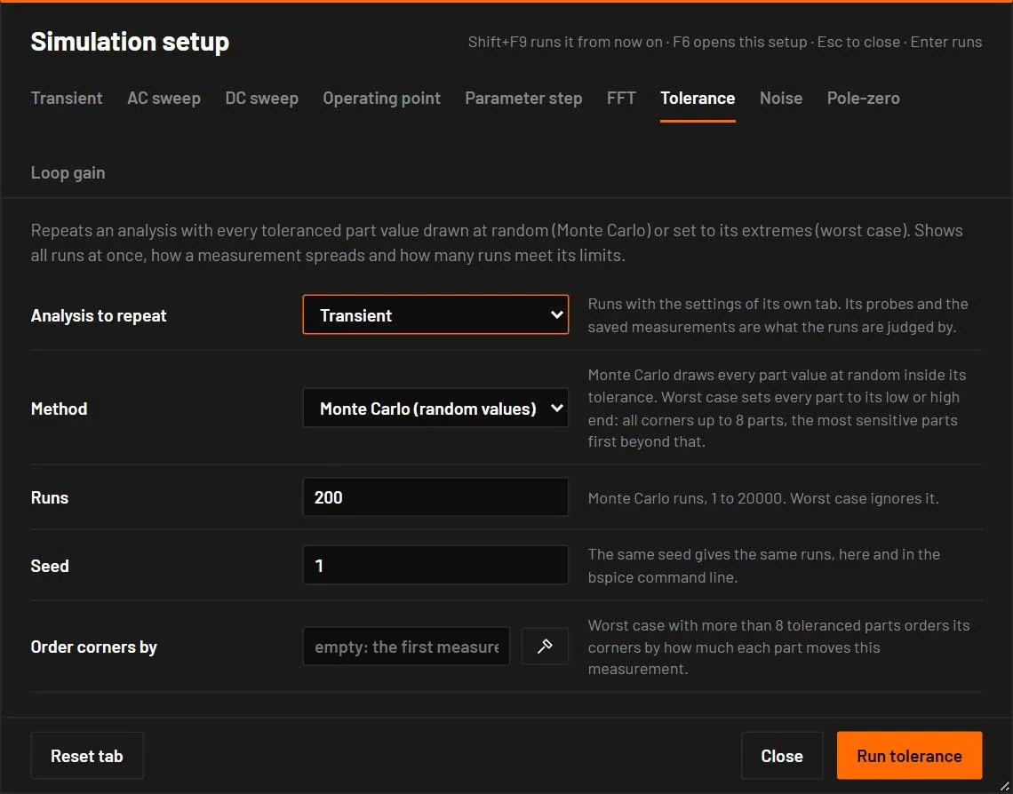
Repeats an analysis many times with the part values changed inside their tolerances. It answers how much the result moves and how many builds would still meet the specification.
Tolerance of a part. Select a part and set Tolerance (percent) in the inspector, and Tolerance distribution under All parameters. Gauss means the tolerance is the 3-sigma limit and a draw is cut at plus and minus 3 sigma. Uniform means every value inside the tolerance is equally likely. The two are saved in the circuit as p.tol and p.tolDist. In this analysis a resistor with no tolerance counts as 1 %, a capacitor as 10 % and an inductor as 20 %. Sources and batteries are exact unless they get one, and a tolerance of 0 makes any part exact. Every other analysis keeps the exact value of every part.
| Field | Values | Default | What it does |
|---|---|---|---|
| Analysis to repeat | Transient, AC sweep, DC sweep or Operating point | Transient | The analysis to run again, with the settings of its own tab. |
| Method | Monte Carlo, Worst case | Monte Carlo | Monte Carlo draws every part at random. Worst case sets every part to its low or high end. |
| Runs | 1 to 20000 | 200 | The number of Monte Carlo runs. |
| Seed | a whole number | 1 | The same seed gives the same runs, here and in bspice. |
| Order corners by | a measurement | the first | Worst case with more than 8 toleranced parts orders its corners by this measurement. |
More parts than resistors, capacitors and inductors have a tolerance of their own, set in the inspector under Accuracy: the input offset limit of an op-amp or comparator (vos_max), the forward voltage spread of an LED or diode (vf_tol), a zener voltage (bv_tol), a regulator output (tol), a crystal frequency (ppm_tol), a transformer ratio (ratio_tol), the 555 threshold and trigger levels, NTC, PTC and RTD resistance, sensor sensitivity and offset, and the offset and gain error of an ADC or DAC. A part is varied only when it sets the value, and an old circuit gives the same runs for its resistors, capacitors and inductors. The full list is in docs/DEVICES.md under Tolerance analysis keys.
Worst case runs every corner (2 to the power of the number of parts) up to 8 parts. With more parts it first moves one part at a time, then sets the most sensitive part, the two most sensitive, and so on, all pushing the chosen measurement up and all pushing it down. That finds the extremes of a smooth response in 4 runs per part. No more than 6 runs go at the same time. The runs use the built-in engine, like a parameter step, and a circuit with vendor models runs with their fitted models.
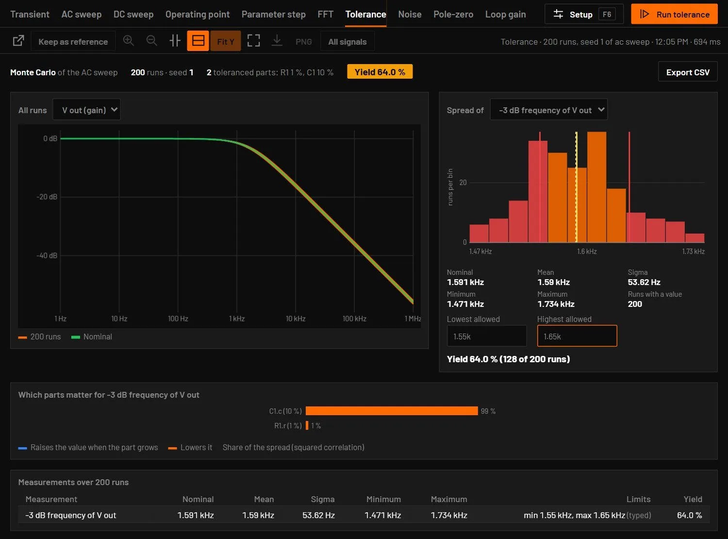
What is judged is the circuit's measurements that fit the analysis (Measurements). A circuit with none uses the final value of its first probes, or the -3 dB frequency for an AC sweep. The result has these parts.
| Part of the result | What it shows |
|---|---|
| The cloud | All runs drawn over each other, with the nominal run on top. |
| Spread of | A histogram of one measurement, marked with the nominal value and the mean, with sigma, minimum and maximum beside it. |
| Yield | Type the lowest and highest allowed value and the share of runs inside shows at once. Limits saved in a measurement start there. A run the engine could not solve counts as a failure. |
| Which parts matter | A bar per part with its share of the spread. For Monte Carlo it is the squared correlation of the part value with the measurement. For worst case it is the change of the measurement when the part goes from low to high. |
| Table | Every measurement with nominal, mean, sigma, minimum, maximum and yield. Export CSV writes one row per run. |
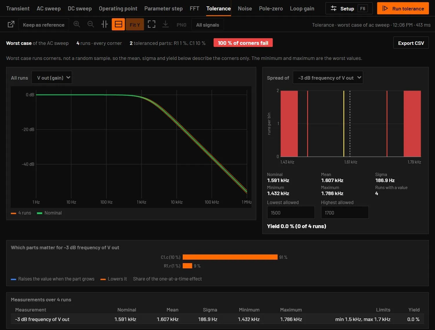
Worst case runs corners, so its mean, sigma and yield describe the corners only. Agents reach this with the tolerance tool.
28.8FFT
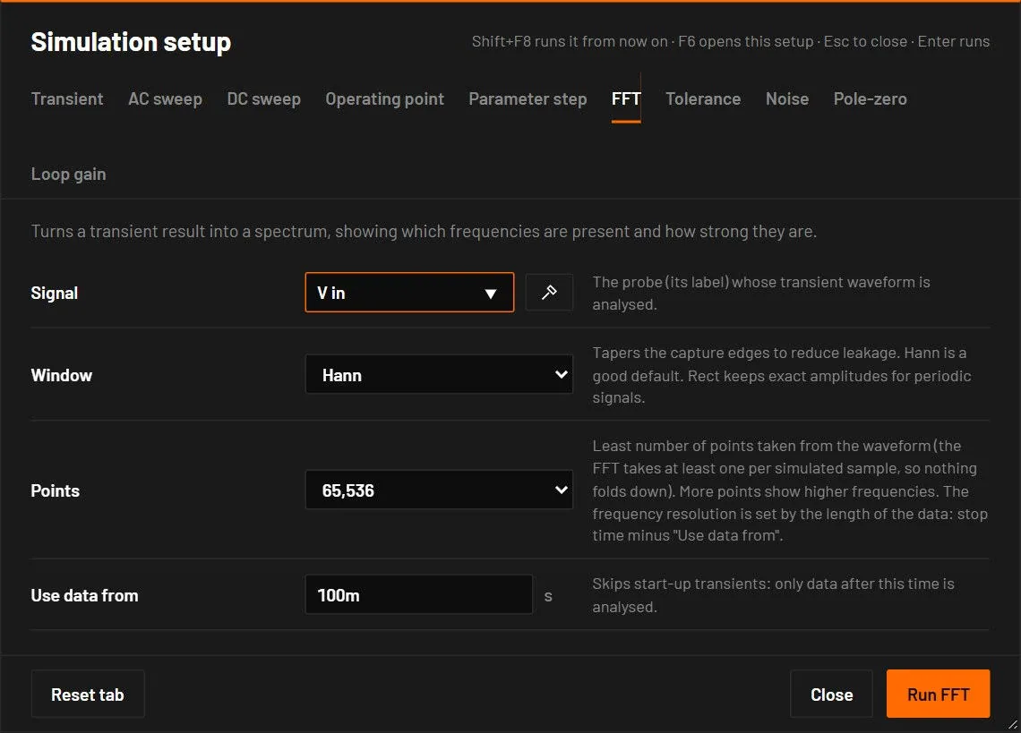
Turns a transient result into a spectrum. The FFT first runs a transient with the Transient tab's stop time and maximum timestep, then analyses one probe.
| Field | Values | Default | What it does |
|---|---|---|---|
| Signal | a probe label | the first probe | Whose waveform is analysed. |
| Window | Hann, Blackman, Rectangular (none) | Hann | The taper against leakage. Amplitudes are corrected for the window: a 1 V sine reads 0 dBV with every window. Rect keeps exact amplitudes for signals that are periodic in the window. |
| Points | 4096, 16384, 65536, 262144 | 65536 | The least number of points taken from the waveform. The FFT takes at least one per simulated sample, so nothing folds down, and past 220 points each point is the average of the waveform over its interval. More points show higher frequencies. The frequency resolution is set by the length of the data: the stop time minus Use data from. |
| Use data from | seconds | half the transient | Skips the start-up. The field warns when it's past the end of the run. At most the first half of the run is skipped. With fewer than 16 samples left the run asks for a longer stop time. |
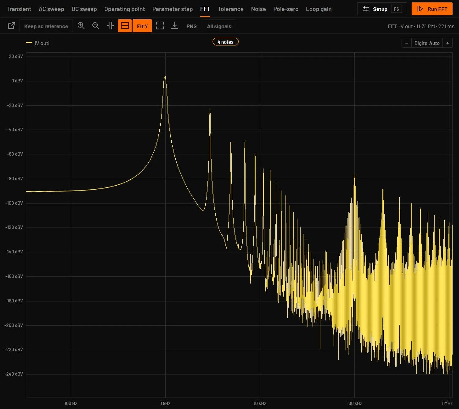
- Open a transistor amplifier example and probe its output.
- Set the Transient stop time to
50m, then press Shift+F8. Window Blackman, Use data from10m.
You should seeThe fundamental stands out with its harmonics below it. Their height in dB below the fundamental is the distortion.
28.9Noise
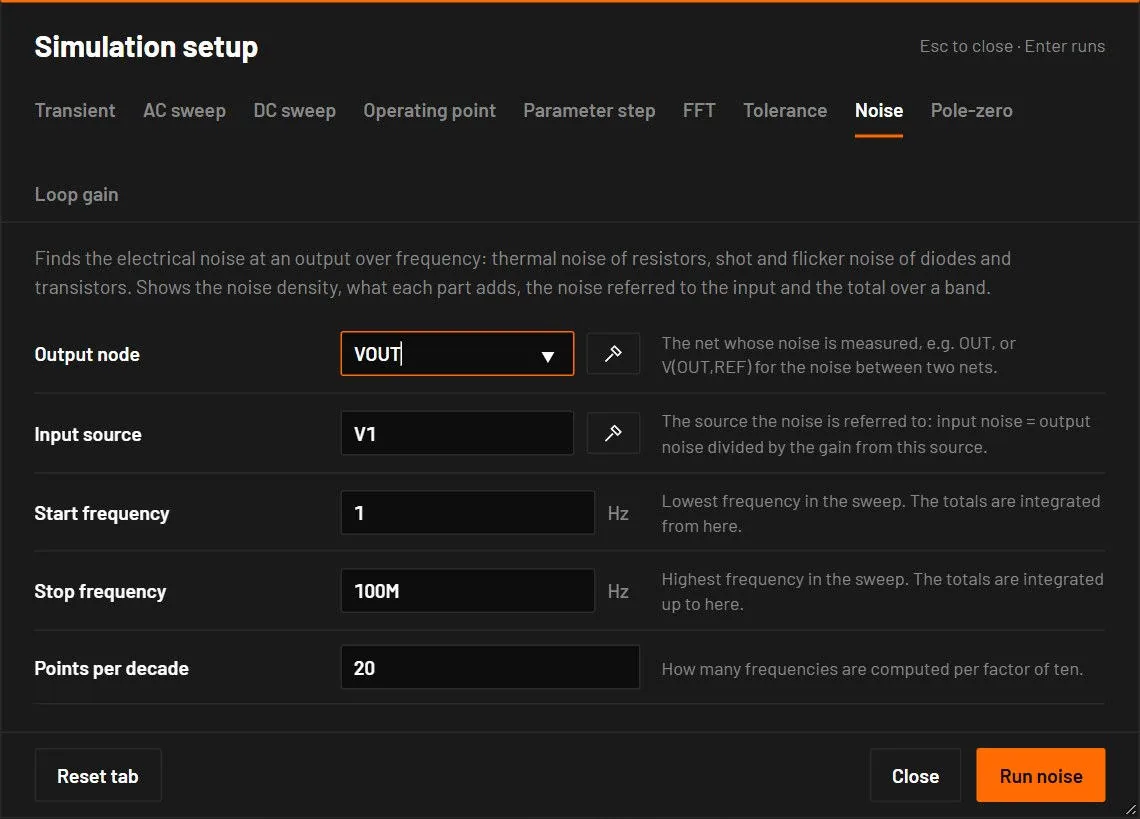
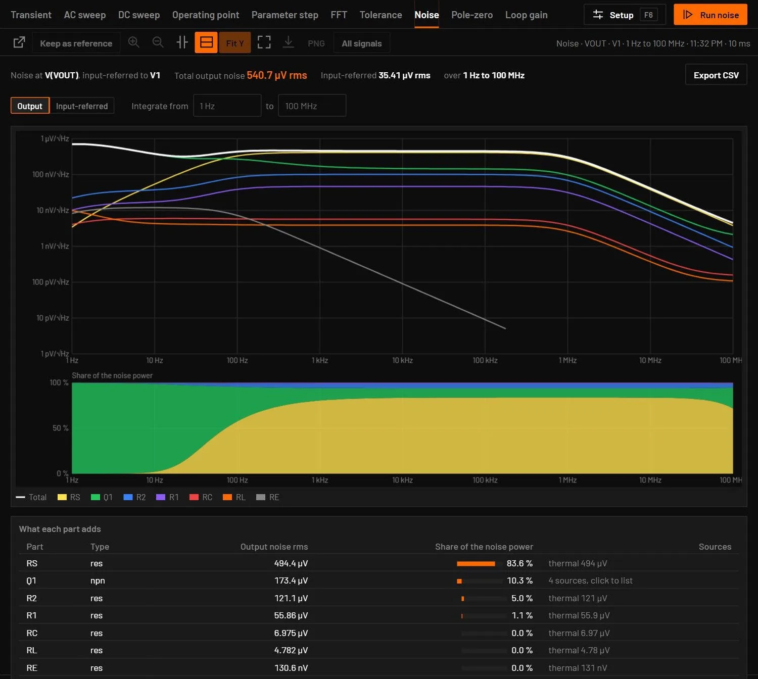
Finds the electrical noise at an output over a frequency sweep. It is the analysis of ngspice’s .noise. Every part with noise adds its sources at the operating point.
| Field | Values | Default | What it does |
|---|---|---|---|
| Output node | a net, or V(OUT,REF) for two nets | Whose noise is measured. The pick on schematic button fills it from a click. | |
| Input source | a source of the circuit | V1 | The source the noise is referred to: input noise is the output noise divided by the gain from this source. |
| Start frequency, Stop frequency | Hz | 1 and 1Meg | The sweep. The totals are integrated over it. |
| Points per decade | whole number | 20 | How many frequencies are computed per factor of ten. |
| Part | Noise it adds |
|---|---|
| Resistor | Thermal noise 4kT/R. |
| Diode, BJT | Shot noise 2qI, and flicker noise KF · IAF / f. RS, RB, RC and RE add thermal noise. |
| MOSFET, JFET | Channel noise 4kT · (2/3) gm and flicker noise. MOSFET levels 1 to 3 follow ngspice’s NLEV (default 2). |
| Built-in op-amp | The thermal noise of its 1 Ω pole node. |
| Ideal sources, capacitors, inductors without resistance | None. A behavioural block with no noise model is named under the table. |
Set KF and AF on a part, or in its model card, for flicker noise. A circuit with vendor models runs in ngspice in the desktop app, so the noise sources inside the vendor subcircuits count. The result shows:
- Total output noise in V rms over the sweep, and the input-referred total (V for a voltage source, A for a current source). Type a band in Integrate from … to and the totals, the table and the shading follow that band. The integration takes the density as a power law between two points, as ngspice does, so 1/f and white noise integrate exactly.
- The density in V/√Hz on log-log axes: the total and each part’s own curve. Input-referred switches the plot to the input. Under it, Share of the noise power stacks what each part adds at every frequency (the six largest, the rest as Other parts). Hold the pointer over the plot for the values at a frequency.
- A table of every part: its rms output noise over the band, its share of the noise power and its noise sources (thermal, rb, ib, ic, flicker). Hold the pointer over a row to mark the part on the schematic.
The result was checked against ngspice-47 on a divider, an RC filter, a common-emitter amplifier, an op-amp amplifier, MOSFET and JFET stages and a diode: the densities agree to 0.005 % and the output totals to 0.003 %. ngspice’s own input-referred total holds the gain of each interval’s upper point over the whole interval, which reads up to 11 % high at 10 points per decade. BetterSPICE integrates the input-referred density itself.
28.10Pole-zero
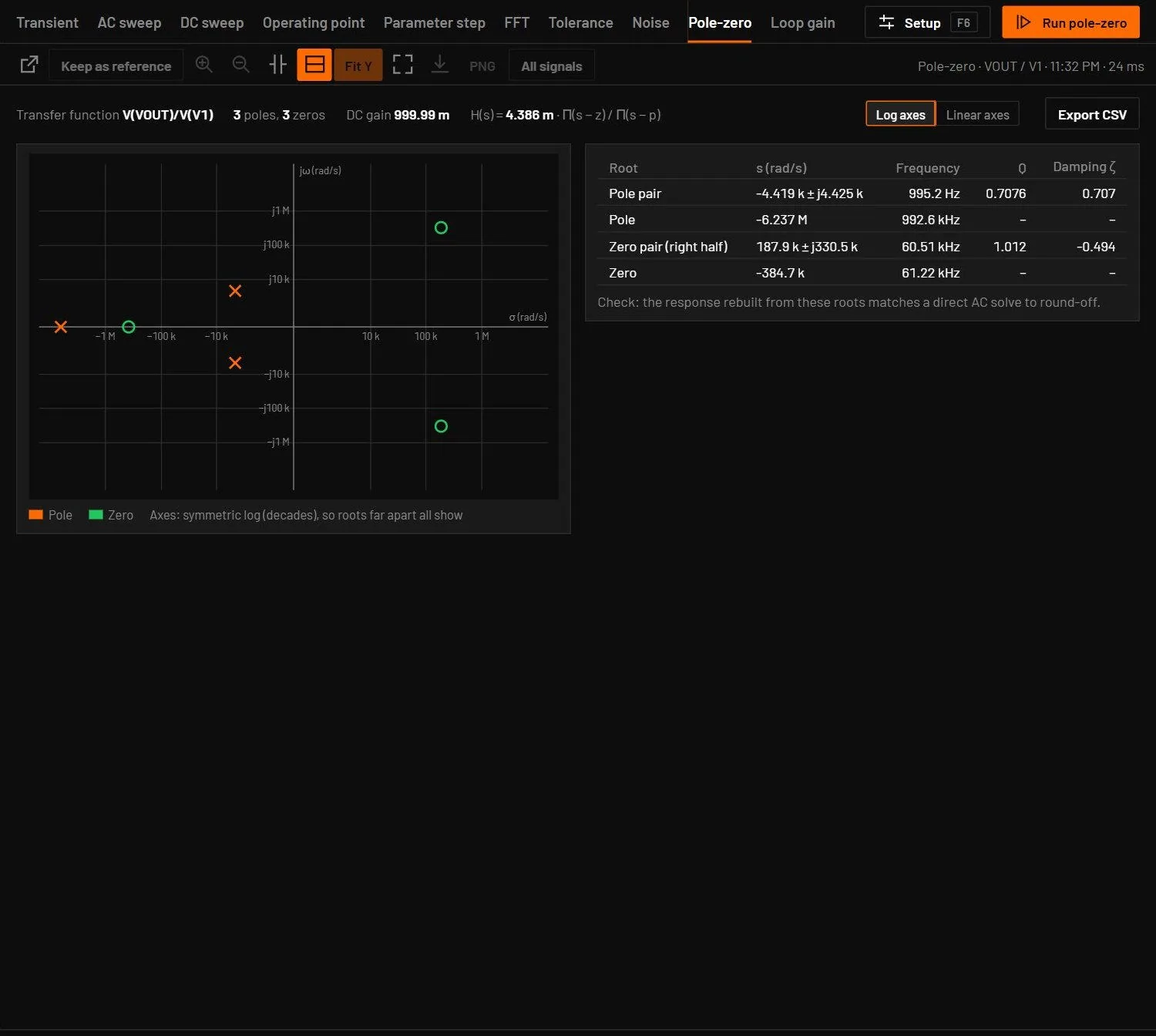
Finds the poles and zeros of the transfer function from an input source to an output node, at the operating point, like ngspice’s .pz. A voltage source gives V(OUT)/V(V1), a current source V(OUT)/I(I1).
| Field | Values | Default | What it does |
|---|---|---|---|
| Output node | a net, or V(OUT,REF) | The output of the transfer function. | |
| Input source | a source of the circuit | V1 | The input: a voltage source gives a voltage gain, a current source a transimpedance. |
The result shows the roots on the s-plane (poles as ×, zeros as ○). Log axes spread roots that lie decades apart and Linear axes show them as they are. The table lists each root in rad/s, its natural frequency in Hz, and Q and damping ζ for a complex pair. A pole in the right half plane is flagged, because the circuit is unstable. The summary gives the DC gain and the constant k in H(s) = k · Π(s − z) / Π(s − p).
The roots are the eigenvalues of the circuit’s small-signal matrices, each refined and checked. The result checks itself: the response rebuilt from the poles, zeros and k is compared with a direct AC solve, and the line under the table says how well they agree. ngspice’s .pz searches for roots one at a time and often gives up on filters and amplifiers (iteration limit reached). Where it finishes, BetterSPICE agrees with it to 10 significant figures. A transmission line has no finite set of poles and zeros and is refused. Pole-zero handles at most 600 unknowns, so run it on the stage that sets the response.
28.11Loop gain
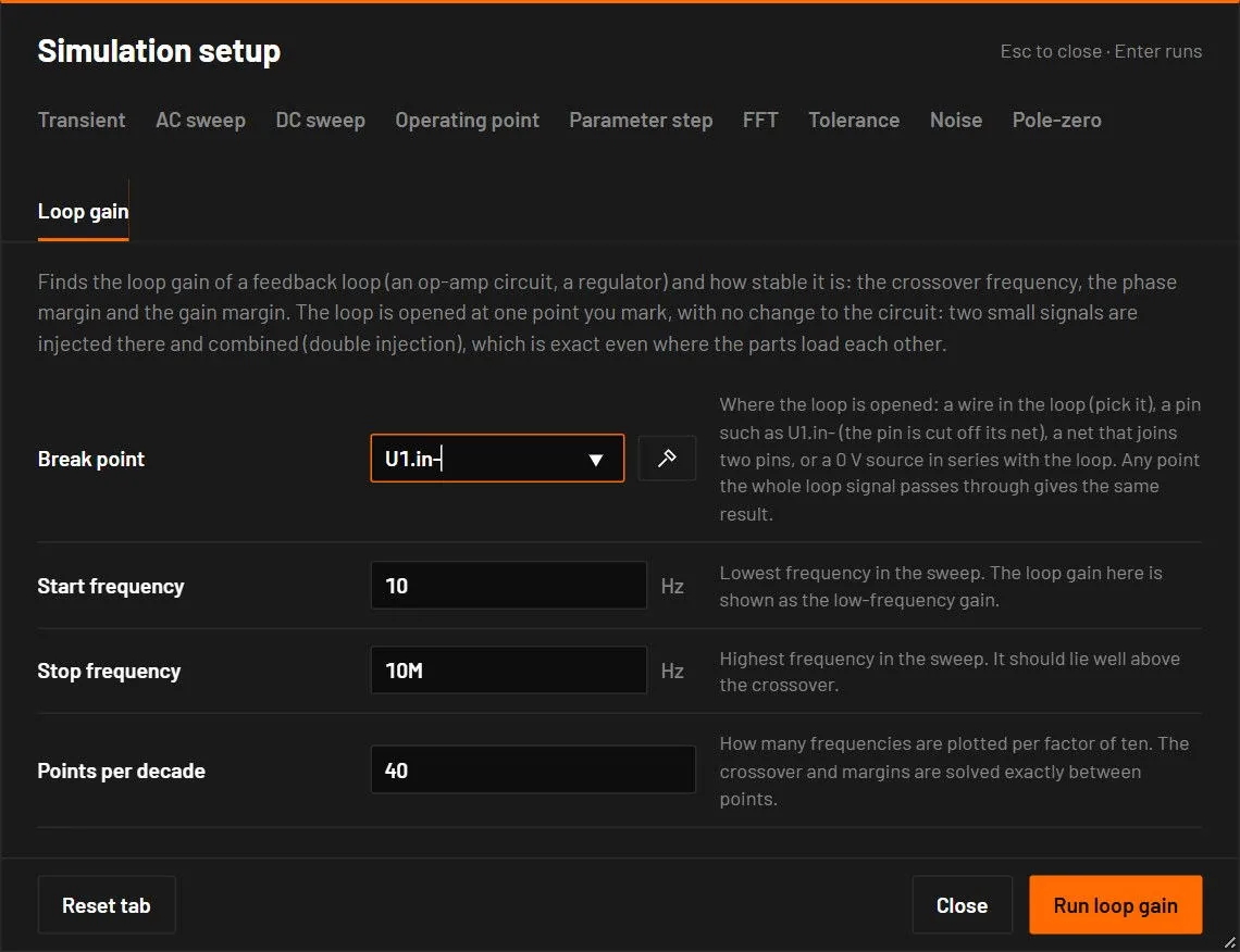
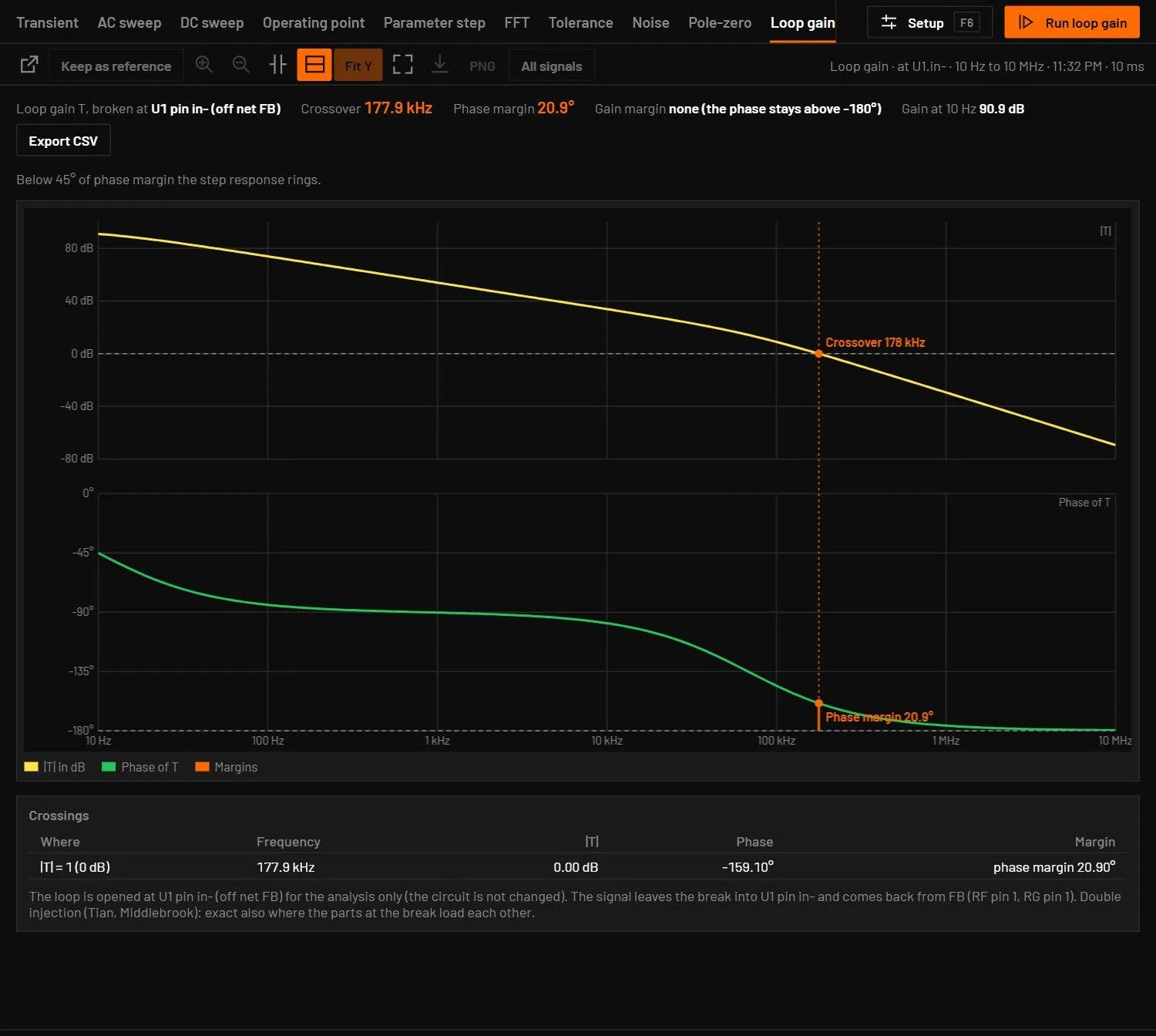
Measures how stable a feedback loop is: an op-amp circuit, a linear regulator, a switching regulator with an averaged or vendor model. It plots the loop gain T(f), the gain a small signal picks up on one trip around the loop.
| Field | Values | Default | What it does |
|---|---|---|---|
| Break point | a wire, a pin, a net or a 0 V source | Where the loop is opened. Press the pick button and click a wire of the loop, or type U1.in- (that pin is cut off its net, the usual choice is the inverting input of the error amplifier), a net that joins exactly two pins such as FB, a 0 V voltage source already in series with the loop such as VINJ, or wire:x,y (what the pick writes). A circuit with a 0 V source in series opens with it filled in. | |
| Start frequency, Stop frequency | Hz | 10 and 10Meg | The sweep. The stop should lie well above the crossover. |
| Points per decade | whole number | 20 | How many frequencies are plotted per factor of ten. The crossover and the margins are solved exactly between points, so they do not depend on it. |
- The crossover is where |T| falls through 1 (0 dB).
- The phase margin is 180° plus the phase of T at the crossover. Below 45° the step response rings, at 0° the loop oscillates.
- The gain margin is how far |T| is below 0 dB where the phase reaches -180°. There is none when the phase never gets there.
- The gain at the start of the sweep, and a table of every crossing. A conditionally stable loop crosses 0 dB several times, and the margins in the header are at the highest crossing.
The circuit is not changed: the break exists only during the analysis. Any point that the whole loop signal passes through gives the same loop gain, and the direction of the break does not matter, because the analysis finds it. At the break it injects a 1 V signal in series and, in a second solve, a 1 A signal into the node, and combines the two (the double injection of Middlebrook, in the form of Tian, Kolar and Middlebrook). Unlike a single voltage injection, which needs a low impedance on one side of the break and a high one on the other, this is exact for any loop, also where the parts at the break load each other. A circuit with vendor models runs both injections in ngspice in the desktop app. An op-amp with a capacitive load agrees with its loop gain worked out by hand to 3e-9 at every frequency, and on four vendor regulator examples it agrees with the AC sweep to 0.001 %. Try the example Loop gain of an op-amp driving a capacitive load in Op-amp circuits.