
Probes, scopes and the dock
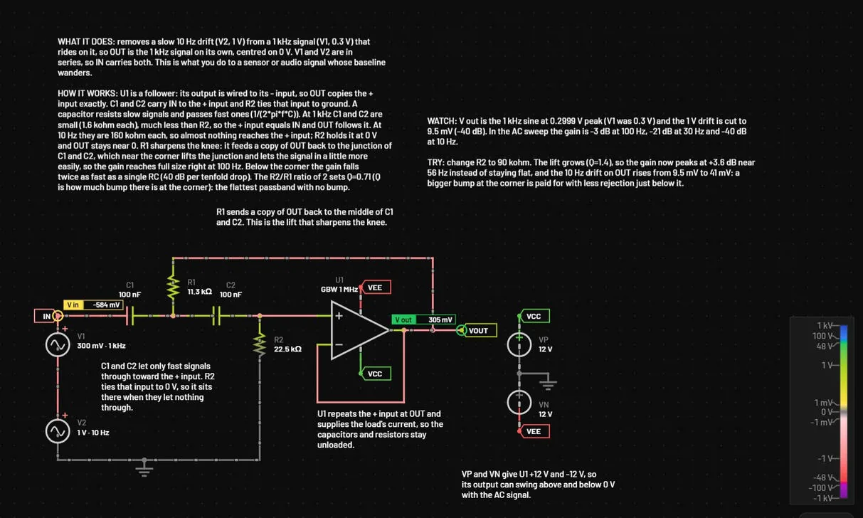
Probes are the signals you want to watch. The scope plots them live, the analyses plot them in the Analysis view, and the report includes them. On the schematic each probe has a tag in its trace colour with its name. A meter probe also shows its value in the tag, all the time (10 updates a second, set with Update in the Measurements header, and while paused the value at the scope's playhead). Place one with the Meter probe tool (Shift+P, the gauge button next to the probe in the toolbar, or Place → Meter probe), or tick Show value on the schematic for any probe: in the inspector when the probe is selected, or in the right-click menu of its name in the scope. Put a tag wherever you want the reading: with the probe tool, click the wire or part where the value should show, and the tag lands there. Drag any tag to move it. Away from its probe, a dashed line joins them. Double-click a tag to put it back beside its probe. Tag positions are saved with the circuit and are part of undo. Probes are saved in the circuit file, can be selected on the canvas and are part of undo.
26.1Probe tags and meter probes
| What | How |
|---|---|
| Place a tag where you want it | With the probe tool, click the wire or part where the reading should show: the tag lands there. A tag is a small box in the trace colour with the probe’s name, and the value when the probe shows it. |
| Move a tag | Drag it anywhere. Away from its probe, a dashed line joins them. Tags follow the probe through moves, rotation and mirroring, and keep their place at any zoom. |
| Name the probe | Double-click its tag. See the next section. Esc during a drag, or switching tab, cancels the drag and nothing moves. |
| Put a tag back | Right-click the probe and choose Tag back beside the probe. |
| Meter probe | Shift+P, or the gauge button in the toolbar. The probe shows its live value in the tag. P gives the plain probe again, and so does Esc. |
| Show value on the schematic | A tick box in the inspector when the probe is selected, and an entry in the right-click menu of the trace name in the scope. A meter probe on a net that already has a probe turns that probe’s value on. |
| Colours | A tag and its ring use the trace colour chosen in the scope, also inside a sheet. |
Tag positions and the value switch are saved with the circuit (the probe’s tag and value) and are part of undo.
26.2Names and colours of probes
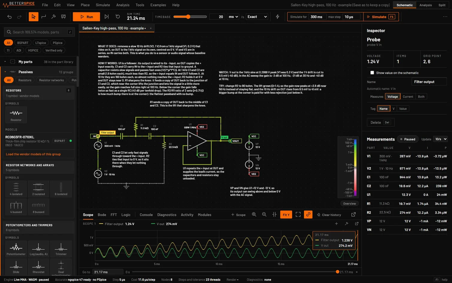
A probe has a name of its own. Type it in the Name field of the inspector, double-click the probe’s tag on the schematic, double-click its chip in the scope or Analysis legend, or choose Name… in the probe’s right-click menu. Clear the field to go back to the automatic name, such as V OUT. A voltage and a current probe that share one tag read V name and I name. Two probes with the same name get a warning in the inspector.
The name shows everywhere the probe does: the schematic tag, the scope legend, the statistics table, the hover card, the CSV headers, the logic analyzer channels, every analysis (transient, AC gain and phase, DC, parameter step, FFT, tolerance and All signals), kept references, the exports and the report. In a measurement the name works as a signal. Renaming updates every view at once and does not run the analysis again.
Each probe keeps one colour, stored with it. Removing another probe never recolours it, and every analysis draws the probe’s traces in that colour. A parameter step draws later values of the step in a shade toward the background. Pick a colour from the swatches in the right-click menu of a trace in the scope. In All signals, an engine signal that a probe reads shows under the probe’s name and colour, and other names read in the scope’s words (V(PWM) as V PWM, I(R1) as I R1).
26.3Adding probes
| How | Probe | Label |
|---|---|---|
| Probe tool P, click a wire | The net voltage to ground, named after the net (a label, or a part pin) | V OUT |
| Meter probe tool Shift+P, click a wire or part | The same probes as the probe tool, with the live value shown in the tag on the schematic | V OUT 4.98 V |
| Probe tool, click near a pin | The voltage at that pin | V U1 pin 2 |
| Probe tool, click the body of a two-pin part | The current through it | I R1 |
| Probe tool, click the lead of a pin of a part with three or more pins (next to the pin, not on its end) | The current into that pin | I Q1 B |
| Right-click a pin of a part with three or more pins, Probe this pin’s current | The current into that pin. On a point the pin shares with another part, that part’s menu offers it as Probe the current into Q1 B | I Q1 B |
| Inspector, Add to scope | The voltage across a two-pin part, or at pin 1 of a one-pin part | V C1 |
| Right-click a part, Add probe | The current through a two-pin part, otherwise the voltage at pin 1 | I C1 |
| Right-click a wire, Add probe (scope) | The net voltage | V net |
| Probe tool on a net of an isolated side | The voltage against that side's own ground (a differential probe) | V OUT (ISO2) |
| Probe tool, Shift+click on an isolated side | The voltage against the main ground GND, even on an isolated side | V OUT (vs GND) |
| Split view, Alt+click a net or part | A trace in the Analysis view, not a saved probe |
26.4A probe for voltage, current or both
Select a probe, or right-click it, and choose Measures: Voltage, Current or Both. Current is offered on a pin of a two-pin part and on a wire with exactly two part pins on it. It is the current into the part's first pin. On a net where several pins meet there is no single current path, so only voltage is offered and the inspector says why.
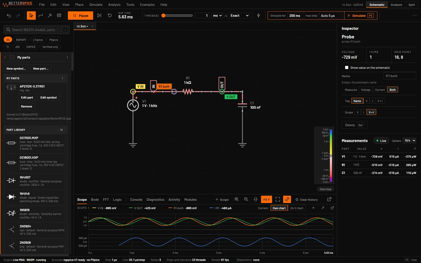
| Setting | What it does |
|---|---|
| Measures | Voltage, Current or Both. |
| Tag | What the tag on the canvas reads: the name, the voltage, the current or both, for example OUT 4.98 V 1.21 A. |
| Scope | Which scope the probe draws in, and whether it draws the voltage, the current or both. |
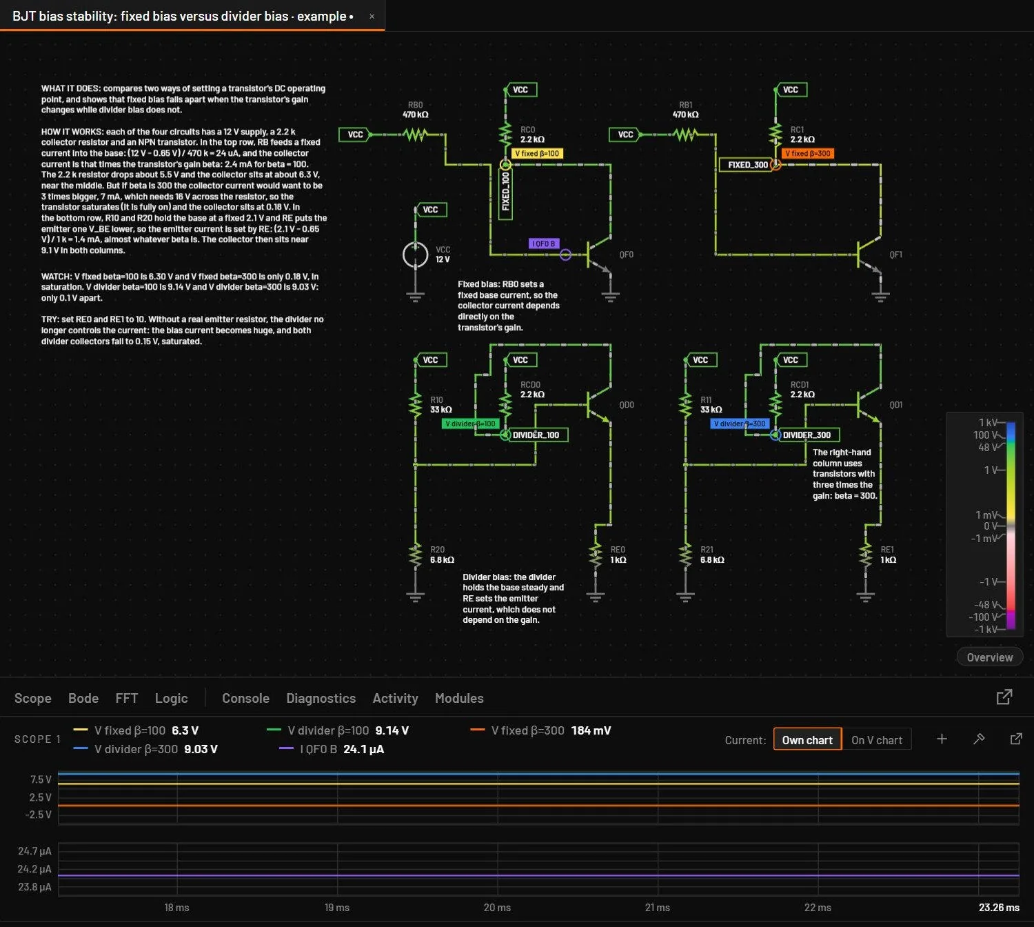
A pin current also works in Simulate for a part with a vendor model: the desktop app puts a 0 V source in series with that pin only for the ngspice run, so the vendor model is not changed. A PSpice run has no pin currents. Neither do a built-in op-amp or transmission line in an ngspice run, because they are written as subcircuits, and a warning names the part.
A probe set to Both puts one trace of each on the scope. With Current: Own chart the amps get a chart of their own. With On V chart they share the voltage chart on a second axis at the right. The Analysis view plots the same quantities. In the file it is two ordinary probes (a voltage probe and a current probe that share a pair), so older builds and older files work as before. In the MCP tools the probe operation takes quantity with "v", "i" or "vi".
Labels follow one rule everywhere: the net's name if it has one (V OUT), else the part and pin (V R1 pin 2), the same words the hover card uses. On an isolated side the probe, the part menu's Add probe and the net menu's Add probe (scope) measure against that side's ground, because a voltage against a ground the side isn't connected to would show the float of the whole side. Capacitors, transformers, optocouplers, solid-state relays, relays and isolators keep their two sides apart, so they aren't joined by a probe. Probing the same pair twice finds the existing probe.
To remove a probe, right-click its name in the scope header and choose Remove from scope (or press Del while that menu is open), click the × that appears when you hold the pointer over the name, or click the probe on the canvas and press Del. Undo brings it back.
26.5The scope
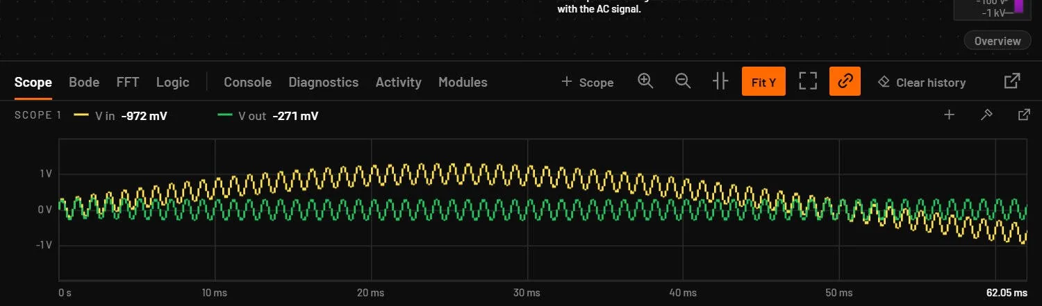
- The scope keeps the most recent 6 seconds of real time. At a timebase of 10 ms/s that is 60 ms of circuit time. The axis shows the time since the run started: it starts at 0 when you press Restart, and the right end shows the time of the newest sample in brighter text.
- Traces of different units on one scope, such as a voltage and a current, get a pane each, with a shared time axis, so both stay readable. A scope that shows both has a Current: Own chart | On V chart switch in its header. On V chart draws the currents over the voltages, with their own scale on a second axis at the right in the current's colour. Own chart gives them their own chart below. The choice is also in the scope menu under Display, and new scopes start with the last one you made. Even a small pane shows at least three labelled values on its axis.
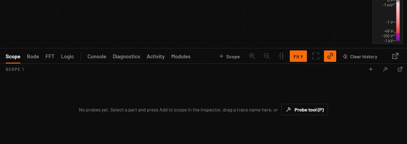
- A scope with no probes shows one line, No probes yet. Select a part and press Add to scope, drag a trace name here, or, and a Probe tool (P) button, with no axes. It still accepts a trace dragged onto it. A scope with no data yet reads 0 … window, never a negative time, and a new run resets each scope's own zoom.
- The header of each scope shows its name, a chip per trace with its colour and latest value, and buttons for adding traces (+), the probe tool, pop out and remove.
- The + button lists every net of the circuit (its voltage) and every two-pin part (its current), with a search box. Click an entry to add it to that scope. An entry with a ✓ is already shown, and a click removes it. Enter picks the first match.
- Click a trace chip to hide or show it. Right-click it for its own menu: Remove from scope, Hide (keep recording), Show value on the schematic, Rename…, its colour, Currents on the voltage chart (right axis) when the scope has both, Move to scope 2 or Move to a new scope, and Spectrum (FFT). Drag a chip onto another scope to move the trace there.
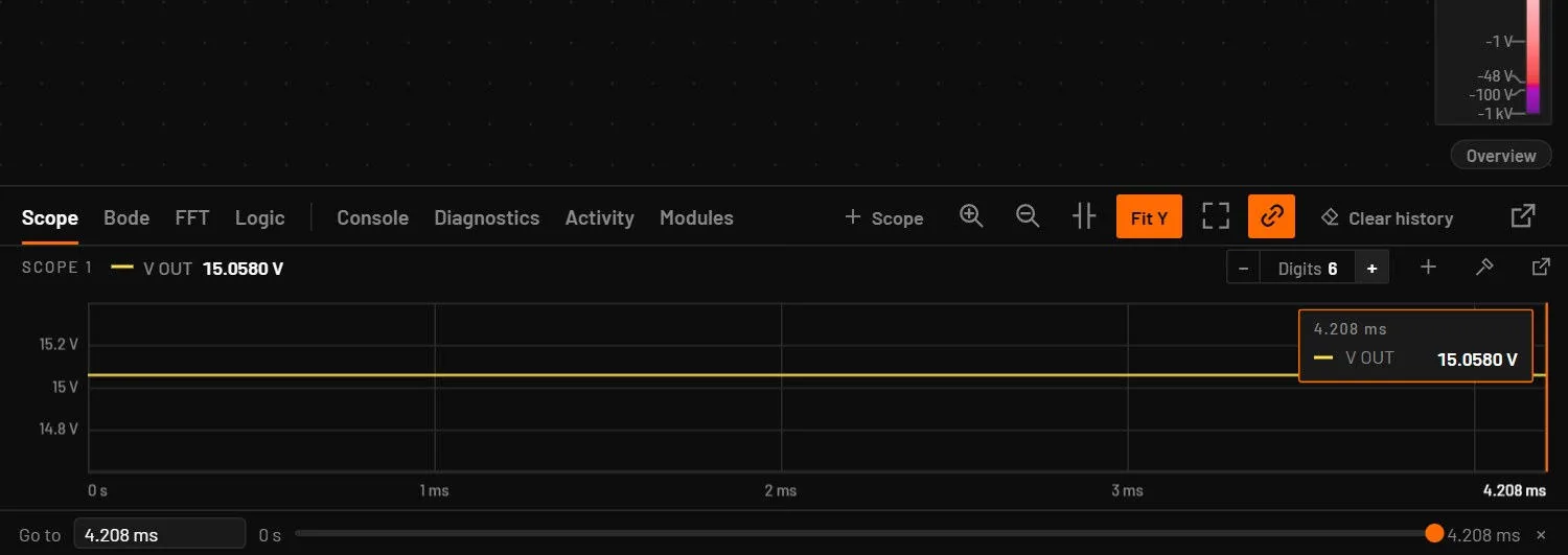
- Hold the pointer over the plot to read every trace at that instant. The readout has one digit more than the axis ticks (2.92 ms against 1 ms ticks). Drag a box to zoom, use the wheel to zoom in time, Ctrl-drag or right-drag to pan, and double-click to reset. Neighbouring ticks never read the same: an ordinary axis gains digits as you zoom in (65.501 ms, 65.502 ms), and when a label would need more than 6 significant digits or would not fit, the base is written once in the corner and the ticks show the offset from it.
- The header has the − Digits Auto + control beside the trace values. It sets how many significant digits the readouts show, from 3 to 9, and is shared with the Analysis view (Axis labels and readout digits). A narrow dock drops the word Digits, and a very narrow one leaves the setting to Readout digits in the scope menu.
- The dock header has + Scope, Zoom in, Zoom out, Cursors, Fit, Link time axes (the chain button, on by default), Clear history (clears the history of all scopes and restarts the auto scale) and Pop out the dock. Zoom, cursors and fit are greyed on a tab with no data yet. When the window is narrow, the dock tabs scroll, with ‹ and › arrows on the side that has more tabs. Each tab's tooltip shows its key.
- With the run paused and the time axis zoomed in, the vertical axis fits the voltages and currents in view, as the Analysis plot does. The Fit Y button in the dock header and Scale, Fit Y to the zoomed view when paused in the scope menu turn this off, which keeps the axis of the whole record. The choice is remembered. While the run is going the scale works as before.
- The corner of a scope shows Hold, Trig ↑ or Trig ↓, Max or Fixed while those options are on.
26.6Probe suggestions
The empty scope of a circuit that has no probes offers up to four key nets to probe. They are chips with a live value each: an output or a labelled net, the switching node, an inductor current and the input rail. The offer sits inside the scope's empty space and is never a pop-up.
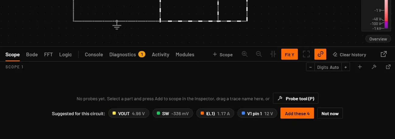
- Hold the pointer over a chip and its net lights up on the schematic. The chip's tooltip says why it was picked.
- Click a chip to add that probe. Add these N adds all of them in one undo step.
- The offer shows once per circuit. Not now, using a suggestion, or adding probes any other way hides it for good.
- turns the offer off for every circuit. Turn it on again the same way.
- A scope with probes is unchanged. The offer shows on the top sheet only.
26.7Several scopes
The + Scope button, or New scope in the right-click menu, adds a scope below. Click a scope to make it the target: new probes go there. Removing a scope moves its traces to the scope above it. Which scope each probe is on is saved in the circuit, so a file with probes on scope 3 opens with three scopes. Each scope remembers its display choices (stacked, stats, scale, trigger and its edge), and Link time axes is remembered too.
With Link time axes on (the chain button in the dock header, on by default), zooming, panning or resetting any scope moves every scope to the same time window, so related signals line up. Turn it off to zoom each scope on its own. Fit returns every scope to the full window.
26.8Scrubbing a paused run
Pause the simulation (Ctrl+R or Pause) and one Go to bar appears below all the scopes. Its ends are the start of the run (0 s after Restart or Clear) and the time you paused. While running, the scopes show only the last screen of time. Once paused they hold the whole run, so you can scrub or zoom out back to the start.
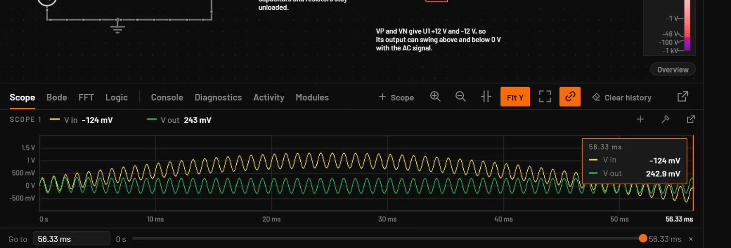
- The playhead starts at the end of the paused run, and Restart clears the paused window and the playhead. Type a time in the box, for example
65.5mor65.5 ms, and press Enter, or drag the slider through the run. - The slider follows the zoom. Zoomed out, a drag sweeps the whole run. Zoomed in, the playhead moves at the scale of the plot, so a drag of one plot width moves it one screen of time. Click the track to jump there. The shaded band on the track, the window the scopes show, can be dragged too. With the slider focused, the arrow keys step (Shift for bigger steps), Home and End go to the ends.
- An orange playhead marks that time on every scope, with a box listing the value of each trace there.
- When the scopes are zoomed in and linked, they centre on the playhead and keep their zoom, so you can step through the run in detail.
- The view stays on what you were looking at when you paused. Double-click a plot, or zoom out, to see the whole run.
- A very long run keeps all of it at a coarser spacing: once it holds 262,144 points per trace it drops every other point, so short spikes from early in the run can be thinner than they were live.
- Drag the playhead line on any plot to move it. The × at the end of the bar removes it. Pressing Run again removes it and the scopes follow the run again.
- Open a circuit with a load step and press Ctrl+R a little after the step.
- Wheel-zoom one scope until the step fills the window: all scopes follow.
- Type the step time in Go to and press Enter, then drag the slider a little either side.
You should seeEvery scope centres on the step, and the playhead boxes show the voltages and currents at each instant.
26.9The scope menu
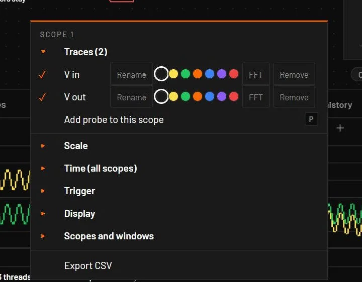
The menu has groups, and one group is open at a time: Traces, Scale, Time (all scopes), Trigger, Display, Scopes and windows, then Export CSV. It fits the window height and scrolls when it must.
| Group | Entry | What it does |
|---|---|---|
| Traces | A tick per trace | Shows or hides the trace. |
| Rename | Renames the trace in place: one undo step. The probe keeps its point, scope and colour. | |
| Colour swatches | One of the six trace colours, or the default (by order). Saved with the probe. | |
| → 2, → 3 … | Moves the trace to that scope. | |
| FFT | Shows the spectrum of that trace in the FFT tab. | |
| Remove | Deletes the probe from the circuit. | |
| Add probe to this scope (P) | Makes this scope the target and starts the probe tool. | |
| Scale | Auto fit | The vertical range follows the data. It grows at once and shrinks only after the traces used less than half of it for a second, so it doesn't jump. Paused, it fits at once. |
| Max hold (grow only) | The range only grows. | |
| Fix current scale | Freezes the range as it's now. | |
| Manual min and max | Type a Min and a Max for each unit shown (volts, amps), for example -5 and 500m. A field left empty follows the auto scale on that side. Min has to be below Max, and nothing changes until it is. The same entry is in the Analysis view's Scale menu. | |
| Readout digits | The − Digits Auto + control: how many significant digits the readouts of every scope and the Analysis view show, 3 to 9 or Auto (Axis labels and readout digits). | |
| Time (all scopes) | Faster (window ÷ 2) / Slower (window × 2) | Halves or doubles the time window. |
| Reset zoom, Clear scope history | ||
| Trigger | Off (free running) | The trace scrolls. |
| Rising edge / Falling edge | Holds the newest matching edge of the source trace at a quarter of the window, at the middle of the trace's range, so a periodic signal stands still. | |
| Source: trace | Click to cycle the trigger source. | |
| Display | Stack traces | One pane per trace instead of overlaid. |
| Show stats (max, min, RMS, freq, duty) | A table per trace with Max, Min, Avg, RMS, P-P, Freq and Duty over the visible window. | |
| Cursors | Cursor lines A and B with a readout. | |
| Hold picture | Freezes the picture while the simulation keeps running. | |
| Scopes and windows | New scope, Move trace to a new scope, Remove scope N | Adds or removes a scope. A removed scope's traces move to a neighbour. |
| Pop scope N out / Put scope N back | Moves the scope into its own window and back. Move scope N to scope window k joins another one. | |
| Pop all scopes out / Pop the whole dock out | All scopes, or the whole dock, in their own window. | |
| Export CSV | Saves the rows in the visible window as scopeN.csv: a time column in run time and one column per trace with its unit. |
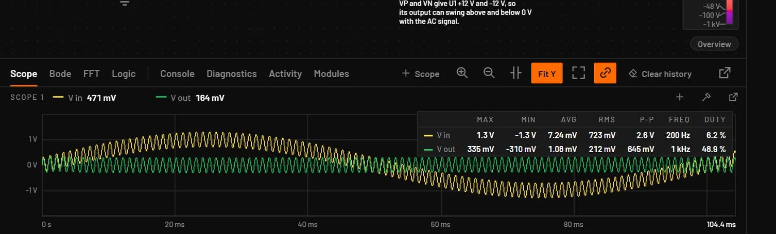
Average and RMS are weighted by time. Frequency and duty cycle are measured at the middle level with hysteresis, and show a dash when the signal has no real swing.
26.10Cursors
Cursors put two vertical lines on the plot, A (solid) and B (dashed), at 30 % and 70 % of the window. Drag a line to move it. The readout on the right lists the time at A and B, their difference Δ and 1/Δ in hertz, and each trace's value at A and B with the difference. The same cursors work in the scope, the Bode and FFT tabs and the Analysis view.
- Open Diode circuits and a bridge rectifier example.
- Probe the output and set the timebase to 10 ms per second.
- Right-click the scope, choose Show stats, then Rising edge in Trigger.
You should seeThe waveform stands still. The stats table shows P-P, the ripple, and Freq, 100 Hz for a 50 Hz full-wave bridge.
26.11Bode tab
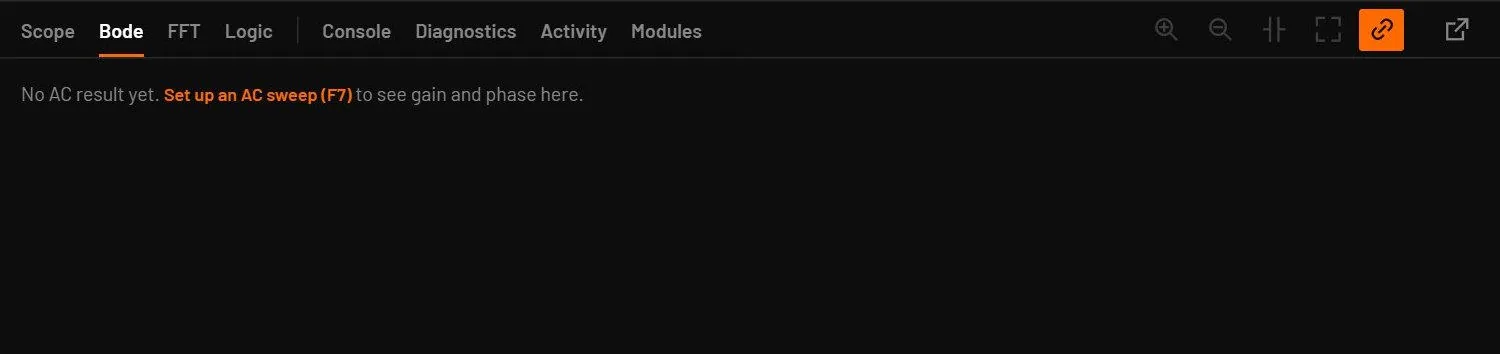
The Bode tab shows the last AC sweep: magnitude in dB and phase in degrees against a logarithmic frequency axis, for the probes. Before any AC sweep it says "No AC result yet. Set up an AC sweep (F7) to see gain and phase here." Zoom and cursors work as in the scope.
26.12FFT tab
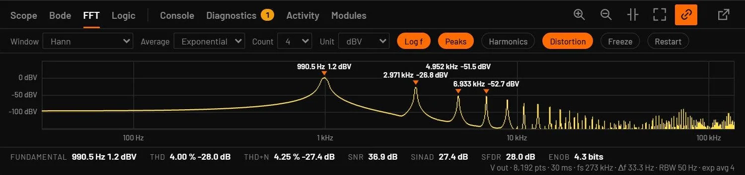
The FFT tab shows the live spectrum of one scope trace, the one chosen with FFT in the scope menu or the first trace. Levels are RMS values, so a 1 V peak sine reads -3.01 dBV in every window. The line under the plot gives the record length, the sample rate, the bin spacing and the resolution bandwidth.
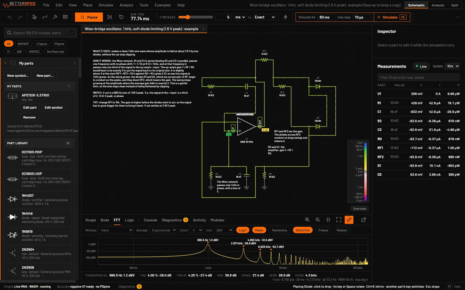
| Control | What it does | Key |
|---|---|---|
| Window | Hann, Hamming, Blackman, Blackman-Harris, flat top or rectangular. | W |
| Averaging | Linear, exponential or max hold, with a count. R restarts it. | A |
| Unit | dBV, dBm into a load you type, V rms or V peak. | U |
| Axis | Logarithmic or linear frequency. | L |
| Peaks | Marks the strongest tones with frequency and level. | P |
| Harmonics | Tags the fundamental and its harmonics. | H |
| Distortion | THD, THD+N, SNR, SINAD, SFDR and ENOB of the strongest tone, which is found automatically. | D |
| Freeze | Holds the picture. | Space |
The keys work with the plot focused. The choices are remembered. The Analysis view's FFT (FFT) reads peak amplitude in its dBV. Use it for the spectrum of an accurate transient.
26.13Logic analyzer
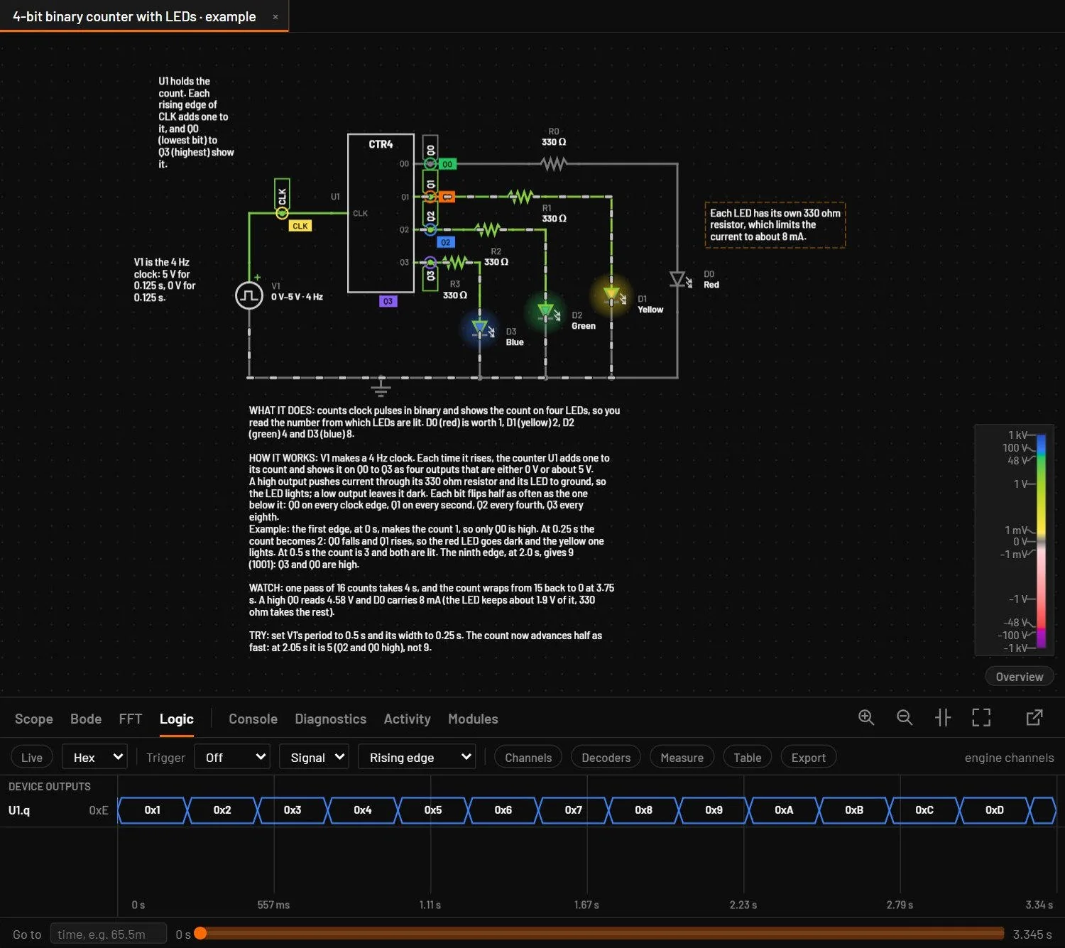
Alt+4 opens the Logic tab, a digital waveform viewer that shares its time axis with the first scope (with linked scopes, with the shared window).
| Group | What appears |
|---|---|
| DEVICE OUTPUTS | The digital outputs of logic gates, flip-flops, counters and control blocks, named like U3.q0, and buses like U2.d. |
| PROBED NETS | Nets you added with Add to logic analyzer… from a wire's right-click menu, labelled D net, read as high or low at the threshold you chose. |
| Control | What it does |
|---|---|
| Live / Hold | Follows the newest sample, or holds the picture. Panning or zooming back to the live end follows the run again. |
| + / − | Zooms time in or out by a factor of two. The dock header has the scope's own zoom in, zoom out, cursors and Fit buttons on this tab. |
| Fit | Shows the whole recording when the run is paused, and the live window while it runs. A double-click on the plot does the same. |
| History bar | Under the plot: the run start and end times, a band for the window you are looking at, and a Go to box. Click the bar to jump, drag the band to scroll through the recording. It works while the run goes and while it is paused, and it sets cursor A. |
| Find | Type a decoded value, as 0x41, 65, b101, a character or some text. Enter goes to the next match and Shift+Enter to the previous one. The matches are outlined and counted. |
| Export | Saves the channel edges as a CSV file. The decoded table has its own Save CSV. |
| Bus format | Hex, Dec or Bin for bus values. |
| Trigger | Off, Normal or Single. Single waits for the next matching edge after you arm it (earlier edges don't count), then pauses the simulation with the window held on that edge and the trigger marker still shown. |
| Signal and condition | The trigger signal and Rising edge, Falling edge, Any change, or Value = with a value box. |
| Clear cursors | Removes cursors A and B. |
| Mouse | Click sets cursor A, Shift-click cursor B (Δt and 1/Δt top right). Drag a cursor line to move it. The wheel zooms about the pointer, and a drag pans. The window cannot go before the first sample or past the live time. |
Buses are drawn as segments with their value, single bits as high and low lines, and unknown states as a red band. Each signal keeps its last 8192 edges. The engine checks a net you added with Add to logic analyzer… against its threshold on every step, so the channel catches every edge the engine computes, however long the scope’s timebase is.
When there are more channels than fit, the channel rows scroll. Turn the wheel over the channel names (over the plot the wheel still zooms in time), drag the bar at the right edge or click its track, or press the up and down arrows or Page Up and Page Down. The decoder lanes and the time axis stay where they are.
26.14Decoders
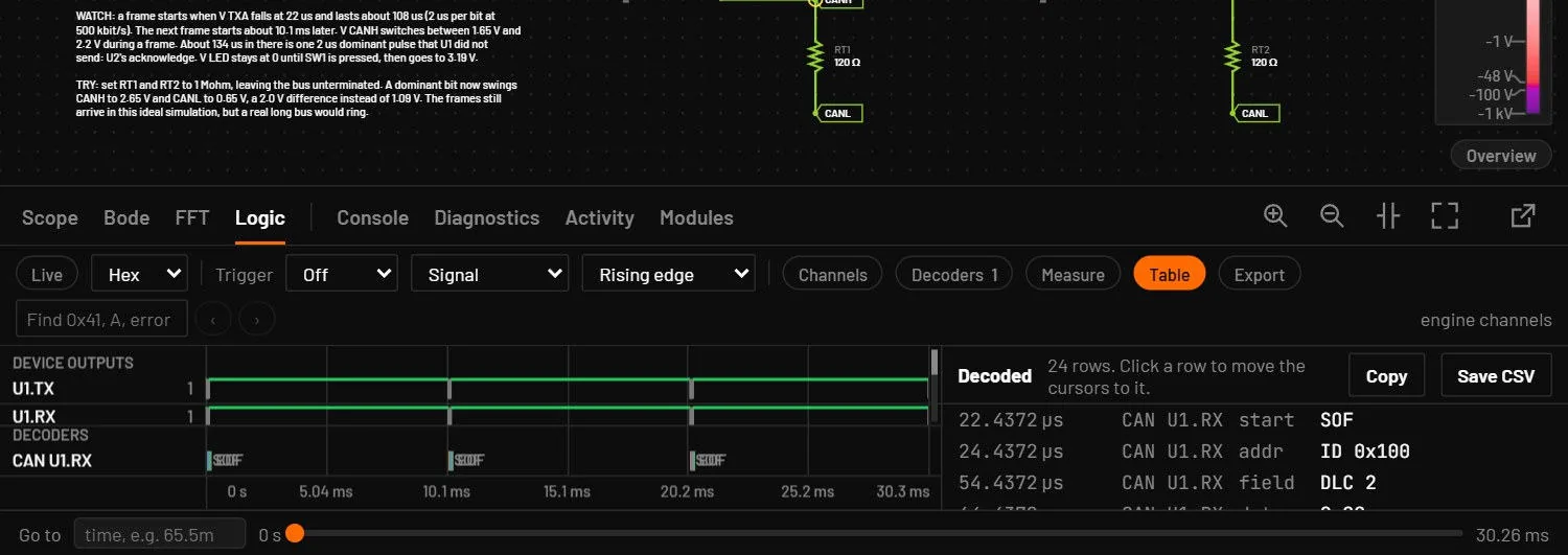
The Decoders button adds a UART, I2C, SPI, CAN, 1-Wire, PWM or Manchester decoder. Pick its channels (a guess is made from the names) and its settings. Decoded frames are drawn over the waveforms in their own lane, and Table lists them with the time, kind and value. Click a row to put the cursors on that frame. Errors are marked in red. The decoders are saved in the circuit, so an example or a shared file opens with its decoded lanes. Save keeps them and Undo takes a change back. The channel names, colours and buses belong to the session.
| Decoder | What it reads |
|---|---|
| UART | Bytes, also as text. Framing and parity errors and a short byte are marked. The baud rate can be Auto. |
| I2C | The 7-bit address, read or write, data, ACK or NACK, start, repeated start and stop. An acknowledge cut off by the end of a recording does not end before it starts. A control block’s own outputs show only what the master drives: to see the slave’s ACK add the net itself. |
| SPI | Modes 0 to 3, with an optional chip select. A clock paused in the middle of a word is marked. |
| CAN | One logic-level line, dominant low: a controller’s RX (the bus as it reads it) or TX. It finds the start of frame on an idle bus, takes out the stuff bits and reads standard (11-bit) and extended (29-bit) identifiers, remote frames, the length, the data bytes and the CRC, which it checks. The ACK slot reads ACK when a receiver drove it, so decode RX to see it: TX shows NACK there, because the sender leaves the slot recessive. Errors are stuff error, CRC error and form error. Bit rate Auto finds the rate from the shortest pulse. Try mcu-can-two-nodes. |
| 1-Wire | The one data line. A low of 480 µs or more is a reset, a low that a device starts up to 300 µs later is its presence pulse (or No presence when none comes), and each time slot is a bit: a low shorter than 15 µs is a 1, a longer one a 0, eight of them a byte, least significant bit first. overdrive uses the faster timing. Try one-wire-reset-presence-pulse. |
| PWM | The duty and the frequency of every period of a pulse train, from one rising edge to the next (the falling edge with active low). |
| Manchester | A line with a transition in the middle of every bit. A rising one is a 1 in the IEEE 802.3 convention and a falling one in the G. E. Thomas convention (pick which). It shows the bits on one lane and words of the length you set on another, and marks a missing mid-bit transition as a violation. The bit rate on Auto comes from the shortest pulse, which is half a bit. Set it when every bit alternates, because then all pulses are a whole bit long. Try manchester-encoder-xor. |
Other controls of the tab: Channels renames a channel, picks its colour or hides it, and several 1-bit channels ticked together make a bus with Group, read in hex, decimal, binary or ASCII. Measure gives the period, frequency, high and low widths and duty of a channel over the window or between the cursors. The trigger takes a value or a pattern such as 5, 0x1F or b10x1, where x is a bit that does not matter. With the plot focused: + and - zoom, the left and right arrows pan, the up and down arrows scroll the channels, L live or hold, C clears the cursors, T the table, H channels, D decoders, M measure and F the next format.
The window always shows the recording. Zooming the running scope keeps the Logic tab live with the scope's time span. It only holds when the scope is paused or zoomed into the past. A held window that has drifted outside the recording (after a long run, a Restart or a scope zoom) goes back to Live by itself. While you haven't set a zoom of your own, the time span widens until the busiest signal shows a few edges, so a slow signal is never an empty lane. Switching to another document tab starts the Logic tab live for that circuit.
- Open Counters and registers and a binary counter example.
- Press Alt+4. Set Trigger to Normal, the signal to the most significant bit and the condition to Rising edge.
You should seeThe picture locks on each rollover of the top bit. Click and Shift-click two edges to read their spacing.
26.15Console
The Console tab shows the lines that programmable control blocks print with log() and that microcontrollers print with print, and their script errors: the clock time, the simulated time, the part and the message. Error lines are red and counted on the tab. Click a line to select the part. It keeps the last 5000 lines, from every circuit you opened in the session. empties it (greyed when it's empty, and the message offers Undo). Programmable control blocks and Programming the MCU describe the scripting.
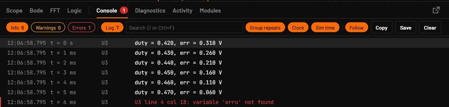
Chips filter the lines by level (information, warnings, errors) and by channel (Log, MCU, Serial). The search box takes words that must all appear, "a phrase", -word to leave lines out and part:U1 for one part. Ctrl+F or / focuses it and Esc clears it. Identical lines in a row fold into one line with a count (Group repeats). Copy (Ctrl+Shift+C) and Save write the lines shown as text, Ctrl+L clears with Undo, and Follow (or End) keeps the newest line in view. Scrolling up pauses it.
The input bar for a USB-UART bridge
When the circuit has a USB-UART bridge (a chip of variant usb_uart, Chips and displays), the Console gets an input bar under the lines. The bridge is the Console's other end: what the microcontroller sends to it shows as lines, tagged with the bridge's designator, and what you type goes out on the bridge's TXD pin to the microcontroller's RX.
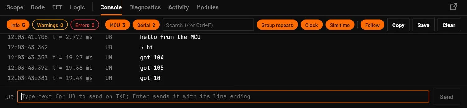
| Part of the bar | What it does |
|---|---|
| Name of the bridge | The bridge that sends. With more than one bridge in the circuit, it is a list: pick the one to send through. |
| Text box | Type text and press Enter, or click Send. The bridge adds the ending set in its Console line ending field (lf by default, or cr, crlf, none) and sends the bytes as 8N1 at its baud rate. |
→ text line | Each text you send is echoed in the Console with an arrow, so the log shows both directions. |
Text goes out only once the live simulation has started (press Play first, otherwise an error line follows the arrow line), and the bridge must be powered (VCC above 2.5 V). A line that reaches the bridge with the wrong baud rate arrives garbled and raises W_UART (Diagnostics and what they mean).
26.16Activity
The Activity tab (Alt+7) lists every edit and run, by you or by an AI agent: the time, the author (you, or the agent's name in violet), what happened and the parts. It includes undo and redo, opening, importing and exporting, runs such as "Ran transient in 42 ms", reloads from disk and take-overs. Click a row to highlight its parts and zoom to them. It keeps the last 2000 entries. (Ctrl+Alt+L) empties it.